ONIs latest White Paper – Fast, high-throughput LNP sizing and characterization using an automated high-precision workflow read here>
Application Kit: LNP Profiler
Last updated: February 12th 2026
This protocol refers to ONI’s Application Kit™: LNP Profiler for capturing and staining LNPs onto the surface of functionalized chips for imaging using super-resolution microscopy.
Sample preparation
Print Section
Component list
| Component | Quantity | Volume | Hazard | Storage upon arrival |
|---|---|---|---|---|
Surface Block | 4 | 55 μL | N/A |
|
Surface Reagent | 4 | 55 μL | N/A |
|
Anti-PEG Capture | 4 | 55 μL | N/A |
|
| Wash Buffer* | 1 | 12 mL | N/A | RT |
| Cargo Detection | 1 | 10 μL | N/A |
|
| PanLNP Detection | 1 | 8 μL | N/A |
|
| Ligand Detection | 1 | 10 μL | N/A |
|
LNP Assay Chip | 4 | N/A | N/A |
|
*Wash buffer can be stored at -20°C, but RT or 4°C is recommended for convenience
Equipment needed
- Pipettes (p10, p20, p200, p1000)
- Pipette Tips (10, 20, 200 and 1000 μL)
- Low Bind Microcentrifuge tubes (1.5mL or 2mL), e.g., ThermoFisher cat # 90410 or similar
- Timer(s)
- Vortex Mixer
- Benchtop microcentrifuge
- Personal Protective Equipment: gloves, goggles, chemical waste disposal
- Aspirator or Vacuum Pump
- ONI Chip Positioner
- ONI magnets
- Humidity chamber
Components to be provided by the user
- Sample to be tested
- PBS without calcium and magnesium for LNP dilutions (as needed)
- Bead slide
Sample Prep Video Tutorial


Step-by-Step Video Guide
Follow along with our ONI team to learn each step of the sample preparation process for the ONI LNP Profiler Application Kit.
Experimental workflow overview
Print Section

Advice before you start
- Launch CSA (CODI System App) and allow the temperature of the microscope to reach 32°C. This will provide ample time for the system to reach optimal temperature. If you are using the Nanoimager please wait for 1 hour, while if you are using the Aplo Scope please wait for 2 hours.
- If prompted to install a new version of CSA, proceed with the install according to the CODI prompts. Remember to reopen CSA after the install is complete.
- Four chips can be prepared in parallel, a pause point is after the antibody detection mix is removed.
- Chips can be stored for up to 24 hrs at 4°C prior to imaging.
- Once cargo detection has been applied to the assay chip, proceed to imaging immediately. Imaging should be completed within 1 hour after the cargo detection incubation is complete. Please consider that imaging using AutoLNP takes 30–50 minutes for each Assay Chip, depending on how many Field of Views are imaged.
- PanLNP Detection, Ligand Detection and Cargo Detection can be freeze-thawed up to three times.
- PanLNP Detection and Ligand Detection reagents can be aliquoted by the user to avoid freeze-thaw cycles, if desired. Do not aliquot Cargo Detection reagent.
Guidance for using the Assay Chip
- Use a p20 pipette for reagent additions, and a p200 pipette for wash steps.
- Assay Chips should be brought to room temperature before opening the pouch and must be used upon opening. Use the chip immediately and do not store opened chips for later use.
- ONI recommends using a designated humidity chamber such as Simport Stain Tray M918-2TM. This will provide three advantages:
-
- a humid environment to avoid evaporation from the lane inlet and outlet,
- protection of the sample from light, and
- avoiding chip movement during pipetting
Humidity chambers can be made with available lab equipment (such as slide storage boxes or dark-colored plastic freezer boxes) provided they meet the advantages listed above.
-
- We strongly recommend the use of a laboratory aspirator to ensure low variability and background within the assay. If you do not have access to an aspirator, use a laboratory dust-free wipe to remove excess liquid, and expect additional variability and additional background in the cargo detection channel.
- Recommended purchasing options for laboratory aspirator:
- Integra Biosciences™ Vacusip Aspiration System
- Grant Bio FTA-1
- Aspeed 2
- Recommended purchasing options for laboratory aspirator:
- The assay surface is VERY sensitive to bubbles or air being introduced to a lane. If transient bubbles are introduced to the lane, you will see increased variability in cluster counts and positivity. If a bubble remains in the lane during an incubation, the region impacted by the bubble will have higher non-specific fluorescent background in all channels and should not be included in analysis.
In order to avoid introducing bubbles, follow these directions:
- Prior to adding a reagent or Wash Buffer to a lane, ensure there is no air in the bottom of the pipette tip. If air is present, gently depress the plunger until you can no longer see the air, and a small drop of liquid is present on the bottom of the pipette tip.
- Firmly place the pipette tip into the inlet (marked “IN”) of the 4-lane chip. Ensure the angle between the pipette tip and chip surface is approximately 90 degrees. A slight flex in the pipette tip indicates a seal has been created.
- If liquid spills out of the inlet, press the pipette tip down harder to ensure a full seal. Remove any spilled droplets with a lint-free lab wipe.
- Apply new reagents and Wash Buffer at a constant rate, depressing the plunger until the first stop.
- Do not pipette past the first stop.
- Watch carefully for bubbles in the pipette tip and stop pipetting immediately if a bubble is about to be introduced to the lanes.
- If bubbles are introduced, wash the lane with 100 μL of Wash Buffer to dislodge them and reintroduce the intended reagent. If the bubble would be washed, mark the area to avoid imaging.
- As you pipette liquid into the inlet hole, the liquid will flow through the lane and exit through the outlet marked “OUT”.
During wash steps only:
- Remove excess liquid as it flows out of the outlet using a vacuum aspirator placed at the bottom of the outlet reservoir.
- Ensure the outlet is empty before reagent addition steps.
During incubation steps:
- Do not use the aspirator. Leave the outlet reservoir full.
- The outlet has sufficient volume and will not overflow.
Use an active aspirator during all wash steps:
- Start pipetting in the Wash Buffer, then place the aspirator tip into the corner between the outlet reservoir wall and lip.
- Continue aspirating as you add the Wash Buffer and stop once the full 100 µL has been added.
Diagram of active aspiration
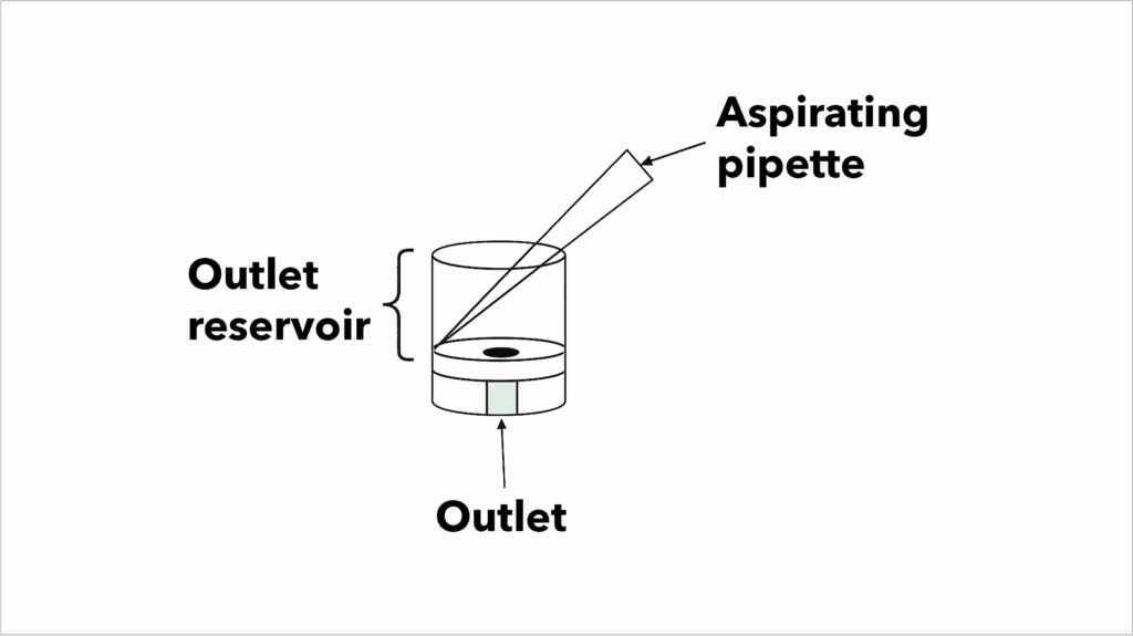

- If a bubble is visible in the inlet after an incubation, CAREFULLY place the aspirator tip on the edge of the inlet to remove this bubble. Do not let the aspirator tip into the inlet, as this will empty the lane.
- At the end of a wash step, the outlet reservoir should appear empty and liquid should remain in the opening below the reservoir.
- If bubbles are introduced during the assay workflow and remain in the lane during a reagent incubation, mark the bubble with a sharpie or take a photo, so that the area can be avoided while imaging.
- If a lane is completely dried out (i.e., air is introduced at the end of a pipetting step, and there is no liquid in the lane), do not image this lane, as the air will negatively impact the assay, primarily impacting non-specific background. Do not include these lanes in analysis.
Stepwise protocol
Print Section
Notes
- Remove the assay chip from the pouch and place it on a clean, dark surface. This will make it easier to see if any bubbles are introduced.
- At the beginning of the assay, all assay components except Cargo Detection can be removed from the freezer and held at room temperature.
- Cargo Detection must be thawed at room temperature for 15 minutes prior to use.
- Allow all reagents to reach room temperature before using. Do not use a reagent if there is still ice in the tube.
- Reagents are meant to be used at room temperature and should not be stored on ice.
- All steps are performed at room temperature.
- All volumes provided are per lane.
- Vortex each reagent for approximately 5 seconds once thawed. Spin down in a microcentrifuge if needed.
- Use a new pipette tip for each lane when adding reagents or washing.
- Outlet reservoir should be full during reagent incubations.
- However, ensure that the outlet reservoir is completely empty at the end of each wash step.
- Always pipette the required solution directly into the inlet hole, marked by “In”.
- Do not tilt the chip, as this can cause flow within the lane.
- Incubate the Assay Chip in a designated humidity chamber or in an appropriate alternative, as suggested in “Guidance for using the Assay Chip”.
- Make sure LNPs stay at optimal storage temperature (4C, -20C or -80C) until completion of Step 5 (Anti-PEG capture)
- Suggestion on pipetting speed – 3-4 seconds to depress plunger to ensure smooth flow
- PanLNP Detection, Ligand Detection, and Cargo Detection can be returned to the freezer after use.
- Do not vortex, flick, or spin down the LNPs. This can result in a fragmented appearance when imaging.
Surface preparation – total time: 40 min
- Add 10 µL Surface Block. [15 min incubation in room temperature, preferably in a humidity chamber]
- Wash with 100 µL of Wash Buffer, using active aspiration.
- Add 10 µL Surface Reagent. [10 min incubation in room temperature, preferably in a humidity chamber]
- Wash with 100 µL of Wash Buffer, using active aspiration.
- Add 10 µL Anti-PEG Capture. [10 min incubation in room temperature, preferably in a humidity chamber]
- Wash with 100 µL of Wash Buffer, using active aspiration.
Note
Only proceed to LNP dilution and subsequent steps once the Anti-PEG Capture has been washed out of the Assay Chip.
LNP capture – total time: 50min
- Dilute LNPs in Wash Buffer or 1X PBS. The exact dilution depends on the sample concentration. Final RNA concentration of dilution should be between 40 ng/ml and 100 ng/ml, assuming an encapsulation efficiency of over 50%.
We recommend performing a dilution titration across the RNA concentration range above using a full Assay Chip (four lanes), run a full LNP Profiler Assay, and select the concentration that gives around 1000-2000 clusters (NIM) or 2000-8000 clusters (Aplo Scope) per single Field of View.
IMPORTANT NOTES:
- Do not vortex, flick, or spin down the LNPs. This can result in a fragmented appearance when imaging.
- Remove LNPs from storage after anti-PEG capture has been washed out. Dilute LNPs immediately, and use diluted LNPs within 5 minutes of diluting.
- When diluting LNPs, we recommend performing two dilution steps if diluting over 1:2000.
- When mixing LNP dilutions, we recommend mixing with 50% of the total solution volume. For large dilution (i.e., 1:500 or higher), mix slowly 10 times by pipetting up and down. For small dilutions, mix slowly at least 3 times by pipetting up and down.
EXAMPLE: If diluting 1:14,000, perform the following:
- Prepare a single 2 ml tube with 999 µL of Wash Buffer or PBS without Mg and Ca (tube 1)
- Prepare another tube with 130 µL of Wash Buffer or PBS without Mg and Ca (tube 2)
- Once LNPs are thawed, add 1 µL of the LNP stock to tube 1. When pipetting the 1 µL from the stock, make sure to pipette to the second stop to ensure that the full 1 µL is ejected, and slowly pipette up and down once to ensure LNPs are mixed.
- Once LNPs have been added to tube 1, use a p1000 pipette with a 500 µL volume, and slowly pipette up and down 10 times to mix the LNPs into solution.
- With a p20 or p10 pipette, take a 10 µL volume from tube 1, pipetting up and down 2 times before pulling out the 10 µL volume. Add this 10 µL volume to tube 2.
- Mix tube 2 with a p200 at 100 µL volume by pipetting up and down slowly two times.
- Tube 2 is your final 1:14,000 LNP dilution. Use within 5 minutes of mixing.
- Add 10 µL of the diluted LNPs to a single lane in the chip. Repeat for each LNP sample.
NOTE: Use a p20 pipette with 10 µL volume. Pipette up and down three times (down, up, down, up, down, up) prior to adding to each lane. Change the pipette tip and proceed to the next diluted LNP sample.
[45 min incubation at room temperature, preferably in a humidity chamber] - If not done at the start of the assay, remove PanLNP Detection and Ligand Detection reagents from the freezer during this incubation, and allow them to reach room temperature.
- Wash with 100 µL of Wash Buffer, using active aspiration.
- Add 10 µL of the diluted LNPs to a single lane in the chip. Repeat for each LNP sample.
NOTE: Use a p20 pipette with 10 µL volume. Pipette up and down three times (down, up, down, up, down, up) prior to adding to each lane. Change the pipette tip and proceed to the next diluted LNP sample. [45 min incubation in room temperature, preferably in a humidity chamber] - If not done at the start of the assay, remove PanLNP Detection and Ligand Detection reagents from the freezer during this incubation, and allow them to reach room temperature.
- Wash with 100 µL of Wash Buffer, using active aspiration.
Staining – total time: 65 min
- Prepare Antibody Detection Staining mix.
IMPORTANT NOTES:
-
-
- Ensure detection reagents are completely thawed prior to diluting.
- Vortex briefly (1–2 seconds) prior to use, and spin down in a microcentrifuge if needed.
- Add the Wash Buffer to the dilution tube first. When adding detection reagents, pipette to the second stop to ensure that reagent is completely ejected from the tip.
- Vortex detection reagent mix for 5–10 seconds after adding all components. Spin down in a microcentrifuge if necessary. Tapping the tube on the bench or quickly flicking is also acceptable if liquid is sitting on the sides of the tube.
-
- Choose option a or b according to your experiment.
a. PanLNP, prepare if you are only interested in LNP size and morphology.
| Number of chips | Wash buffer | PanLNP detection |
|---|---|---|
| 1 | 48.75 μL | 1.25 μL |
| 2 | 97.5 μL | 2.5 μL |
| 3 | 146.25 μL | 3.75 μL |
| 4 | 195 μL | 5 μL |
b. PanLNP + Ligand, prepare if you are interested in LNP size, morphology, and the presence of a ligand on your LNPs.
| Number of chips | Wash buffer | Ligand detection | PanLNP detection |
|---|---|---|---|
| 1 | 46.75 μL | 2 μL | 1.25 μL |
| 2 | 93.5 μL | 4 μL | 2.5 μL |
| 3 | 140.25 μL | 6 μL | 3.75 μL |
| 4 | 187 μL | 8 μL | 5 μL |
- Apply 10 μL of Antibody Detection Staining mix to each lane in your chips. [45 min incubation in room temperature, protected from light in a humidity chamber]
- During this incubation, allow the Cargo Detection reagent to reach room temperature for at least 15 minutes before use. Vortex thoroughly, and spin down in a microcentrifuge after thawing.
- Wash the Antibody Detection Staining mix with 100 µL of Wash Buffer, using active aspiration.This is a pause point. Chips can be sealed with the provided stickers, and stored at 4C° in a humidity chamber for up to 24 hours before proceeding to the next step.
- Prepare Cargo Staining mix
- Prepare Cargo Staining mix. Prepare the Cargo Staining mix directly before you plan to image the chip. Prepare 1 chip at a time. Keep the other chips with Wash Buffer in the humidity chamber at 4C°
- Cargo Detection reagent can be held at RT for up to 4 hours, but the Cargo Staining mix has to be prepared fresh for each Assay Chip.
IMPORTANT NOTES:
- Vortex Cargo Detection reagent for 10 seconds once thawed.
- Always add Wash Buffer to the dilution tube first, and then add the Cargo Detection reagent.
- Pipette to the second stop to ensure that reagent is completely ejected from the tip.
- Cargo Detection should change the solution color to a very pale yellow. Thoroughly vortex the Cargo Staining mix until it is a single, uniform color and no Schlieren lines are visible.
- Use Cargo Staining mix within 5 minutes of preparation.
| Number of chips (4 lanes) | Wash buffer | Cargo detection |
|---|---|---|
| 1 | 48.5 μL | 1.5 μL |
- Apply 10 μL of Cargo Staining mix to each lane. [15 min incubation in room temperature, protected from light in a humidity chamber]
NOTE: During this incubation, complete experiment setup and channel mapping in AutoLNP. If you are using Aplo Scope, complete the Laser Power Optimization (see AutoLNP user guide) - Wash with 100 μL of Wash Buffer, using active aspiration. Repeat one additional time.
- Add additional Wash Buffer to fill the outlet reservoir.
- Seal the inlet and outlet of the chip with the provided stickers. Image immediately.
Imaging (30-50 minutes/chip)
Once your chip is ready to image, please proceed to the Nanoimager. If channel mapping has not yet been completed, complete channel mapping prior to placing your chip on the stage.
For further guidance on imaging and analysis with AutoLNP, please refer to the AutoLNP user guide.
Troubleshooting
Print Section
Low or variable capture
I am experiencing low or variable capture of my LNPs
- If LNP capture is low, try increasing the concentration of LNPs applied to the chip.
- To ensure that LNP capture is reliable across experiments, please dilute your LNPs in an identical manner for each experiment, and mix them in an identical manner.
- Prior to introducing 10uL of dilute LNPs into the sample, gently pipette the diluted LNP mixture up and down 3x, and then immediately add 10uL directly to the chip using the same pipette chip. Change the pipette tip and repeat this process for each lane.
- If performing serial dilutions, try carrying over a larger volume from the previous dilution. I.e., if you were using 10uL from dilution 1 for a second dilution, increase the amount of dilution 1 to 100uL (scaling the second dilution appropriately).
- ONI recommends performing no more than two dilution steps.
- Ensure you are using low bind microcentrifuge or PCR tubes to avoid the possibility of LNPs binding to the sides of the tubes.
High background signal
I am experiencing high background signal in the Cargo Detection channel
- High background signal in the Cargo Detection channel will often appear as a blanket haze across the entire FOV.
- Always ensure that you are vortexing the Cargo Detection reagent for a minimum of 10 seconds after it is completely thawed.
- Always vortex the Cargo staining solution prior to adding it to the chip. This ensures that the Cargo Detection reagent is well mixed with the Wash Buffer.
- If this is only present in a subset of FOVs, the most common cause is the introduction of air during a pipetting step. During your assay chip preparation, please follow all the directions in the “Guidance for using the Assay Chip” section, taking care to inspect your pipette tip for any air at the end of the tip prior to introducing a solution into the lane.
- If this phenotype is present across all FOVs in a lane, this may indicate that the Cargo Staining solution was not completely removed after the incubation was complete. Ensure that you are using the active aspiration technique described in the “Guidance for using the Assay Chip” section, and that you perform 2x 100uL washes after the completion of the Cargo Staining step (step 17).
- If high Cargo Detection background continues to occur after the above troubleshooting steps, please contact ONI support with the lot number of your Assay Chips for further assistance.
Variable capture across a lane
I am experiencing variable capture across a lane (i.e., the top half of the lane has significantly more capture than the bottom half)
The default 6 FOVs in AutoLNP have been selected to optimize for capture consistency. If you are not using the default FOVs, please select FOVs within the same region of the chip for the most consistent capture. If you are still experiencing variability across the lane, please refer to the steps for “I am experiencing low or variable capture of my LNPs”.
LNPs not formulated in a PBS-based buffer
My LNPs are not formulated in a PBS-based buffer. Can I use another buffer for diluting my LNPs?
We cannot guarantee that the assay will perform in an ideal manner when used with non-PBS based buffers. You can test if LNPs diluted in PBS vs another buffer result in similar metrics and morphology.
Less than 1000 LNPs/FOV
I have less than 1000 LNPs/FOV. Can I use this analysis?
We recommend only using FOVs that have over 800 LNPs/FOV for further analysis, in order to ensure that the resultant data is reliable.
Low signal
AutoLNP is a CODI application that connects the Nanoimager to ONI’s CODI cloud-based analysis platform, enabling lipid nanoparticle (LNP) characterization using the ONI Application KitTM: LNP Profiler. AutoLNP consists of several advanced features that allow users to perform super-resolution imaging and analysis of an entire 4-lane LNP Profiler chip with reduced hands-on time and a robust pipeline.
Nanoimager Requirements
- Requires active internet connection on Nanoimager PC
- Requires a standard Nanoimager configuration:
- Lasers: 488, 561 and 640
- Nanoimager Mark III (contact ONI if unsure)
Experiencing bright spots
I am experiencing bright spots in the Cargo Detection channel that do not have a PanLNP signal associated with them.
Artifacts occasionally arise during chip manufacturing that can bind to our cargo dye, resulting in bright blue spots in the field of view (FOV). These artifacts do not affect the LNP Profiler assay metrics, including cargo and ligand positivity or associated morphological measurements such as size. Our analysis workflows use machine learning–based algorithms specifically designed to exclude these spots from analysis. While we continue to minimize their occurrence, their presence has no impact on the integrity of your characterization results.
AutoLNP for Nanoimager
Print Section
Overview
AutoLNP is a CODI application that connects the Nanoimager to ONI’s CODI cloud-based analysis platform, enabling lipid nanoparticle (LNP) characterization using the ONI Application KitTM: LNP Profiler. AutoLNP consists of several advanced features that allow users to perform super-resolution imaging and analysis of an entire 4-lane LNP Profiler chip with reduced hands-on time and a robust pipeline.
Nanoimager Requirements
- Requires active internet connection on Nanoimager PC
- Requires a standard Nanoimager configuration:
- Lasers: 488, 561 and 640
- Nanoimager Mark III (contact ONI if unsure)
Prior to using AutoLNP
Placing the chip holder on the Nanoimager
AutoLNP comes with a handy chip holder that makes Nanoimager feel like it was made for LNP Profiler chips. It also allows AutoLNP to know where each lane is without any further specific calibration.
Warning
With the Nanoimager still switched off, place the chip holder on the Nanoimager before opening the CODI System App (CSA).
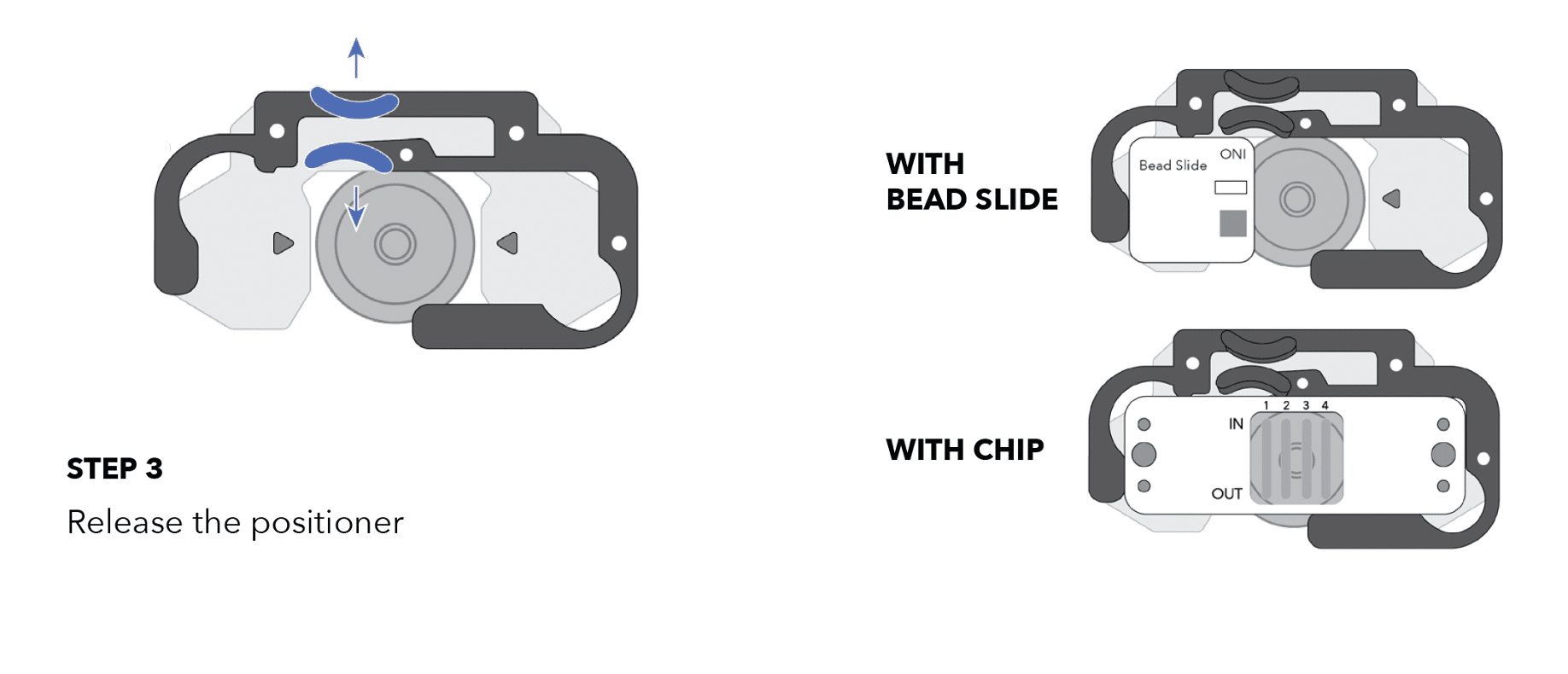
- Place the chip holder on the Nanoimager stage as shown in the illustration below.
- Place the LNP Profiler chip or bead slide (with magnets) inside the chip holder.

Installation & temperature setup

To run the LNP Profiler kit, you will need to register to ONI’s CODI software platform, download the CODI System App and use AutoLNP app.
Navigate to https://alto.codi.bio to access the CODI platform, and make sure to sign and log in, see [1] on image above. If this is the first time creating an account in CODI, contact ONI to get the AutoLNP app activated. Once logged in, look for the microscope temperature control [2], and the Application apps [3] where AutoLNP can be accessed.
Go to Application apps, and select the AutoLNP app. If this is the first time downloading the CODI System App, click “download” as shown in the popup message. Follow the instructions to install the CODI System App.
⚠️ If a “Windows Security Alert” appears, “allow access” to ensure that AutoLNP functions correctly.
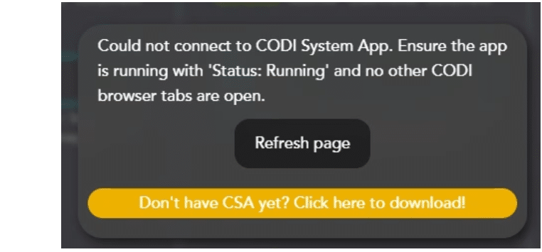
Once installed, open CODI System App and wait for the status indicator to change from “Initializing” to “Running”. CODI System App starts heating the Nanoimager as soon as the application is opened. Click the “Refresh Page” button to close the popup widget.
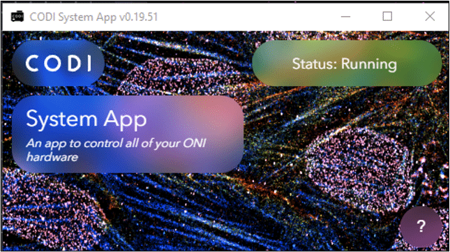
Key Tip: Ensure that the CODI System App is displaying “Running” prior to running AutoLNP, to ensure that the Nanoimager communicates properly with CODI.
Setting a default Nanoimager temperature
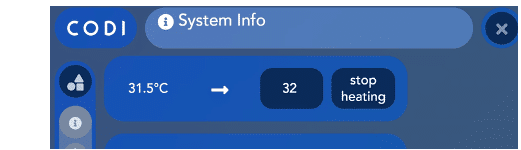
In the top right corner of the CODI page [2], click on the temperature icon with a blue background, which will bring the System Status App, where users can set the desired temperature. This will be saved as the default temperature for the next time the CODI System App is launched. For LNP Profiler, the default recommended is 32°C. Whenever the CODI System App is launched, the Nanoimager will automatically start heating to 32°C and it takes 60 minutes to stabilize and be ready for imaging.
Key Tip
Do not start imaging before the temperature is stable. Any acquisition done during the heating process, will result in a lot of drift. See channel mapping section for more details.
AutoLNP acquisition app
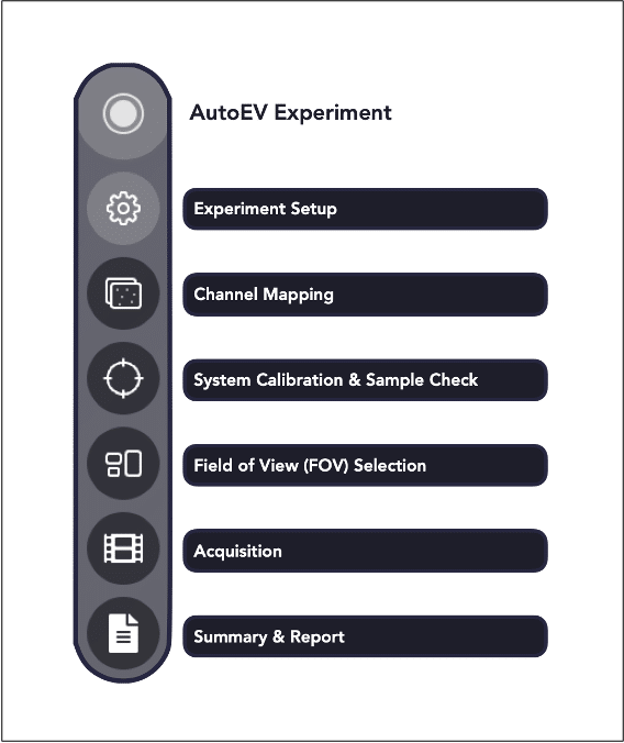
AutoLNP is a linear workflow that helps guide users through the acquisition of the LNP Profiler kit, from experimental setup to acquisition summary. Each step of the workflow has a dedicated page, which can be accessed from the toolbar on the left hand side of CODI.
Move between the pages either by clicking on the individual tabs, or by using the action button on each page to proceed to the next step, e.g., Next, Run, Start acquisition etc.
Experimental setup
- AutoLNP experiment title (chip/sample name):
Give the experiment a name. The datasets will be saved both locally (C:/data/CODI) and on CODI using this name—pick a good one! - Dataset tags: Tags and Key/Value Tags (optional):
Add tags to help distinguish datasets on CODI. Make sure to click the Save button to save any changes. - Collaboration in CODI:
Select a collaboration in CODI where the data will be saved, or use the + button to create a new collaboration.Note: Saving to a Collaboration from AutoLNP is required. - Analysis settings:
The default “AI LNP Profiling” settings are optimized using multiple LNP types. These can be adjusted as needed to suit different analysis needs. - Experiment Settings:
Optimal experiment settings (e.g., channel names, laser powers, number of frames, and exposure times) are preselected.Note: Ensure settings are properly calibrated for each instrument by measuring laser power in mW and adjusting as needed. See Appendix 1 for details.

Data and analysis settings
AutoLNP automatically uploads the data to the selected CODI account and saves it locally in the C:/Data/CODI/ folder. The acquisition data is saved in subfolders with names corresponding to the Experiment and Lane titles provided on this screen.
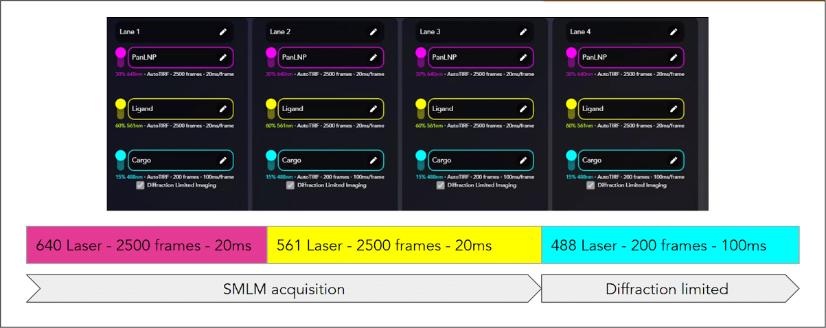
Sample and acquisition settings
Setting up the acquisition to mimic the LNP Profiler Assay Chip with a 4-lane design.
- Enter a Lane Title that represents the LNP sample in that lane (e.g., LNP1 standard control, negative control, or the sample name).
- The channel name field can be edited to match a specific cargo or ligand name.
- For LNPs with both cargo and ligand, leave all channels on. If the LNP sample lacks cargo or ligand, switch that channel off using the vertical slider on the left.
- AutoLNP first acquires the PanLNP using the 638 channel in SMLM mode, then the Ligand in the 561 channel (SMLM), and finally the Cargo in the 488 channel (DL).

AutoLNP provides default starting settings recommended for running the LNP Profiler protocol. Adjust the acquisition settings by clicking on the small text below and input:
- Laser powers need to be adjusted for each user prior to starting an experiment. This may vary depending on the system. Contact ONI if additional information is needed after installation. Laser power values can be updated in the AutoLNP experiment settings page and saved using the Save Current Settings button. See Appendix I for a guide on how to adjust the laser power.
AutoTIRF automatically finds the optimal illumination angle for LNP imaging by maximizing the signal to noise ratio of the spots with respect to the background. The TIRF angle can be manually input in the System Info app. See the “Check TIRF angle” sub-section under the “Calibration & Sample Check” section to select the optimal TIRF angle. - Using the default settings for the number of imaging frames and exposure duration is recommended, as they were optimized for this kit. However, these can be adjusted on a per-channel and per-lane basis if needed.
Applying modified settings across all lanes
AutoLNP has a couple of options to simplify the process of applying the settings to all lanes.
Input the settings in lane 1, then use the buttons at the bottom of that lane to:
- Apply all settings: synchronize all sample and acquisition settings to all lanes
- Apply imaging settings: synchronize only the acquisition settings (channel and lane names will not be synchronized)
- Reset settings to default: reset all lanes to the default LNP Profiler Kit protocol recommendations

Save your own experiment settings
If the imaging settings are updated, such as number of frames or laser power, these can be saved by clicking Save Current Settings. These can be loaded again using Load Settings.
Note: Settings are saved locally on the Nanoimager laptop only and NOT saved on CODI. If web browsers or users are changed, settings will need to be reentered and re-saved.
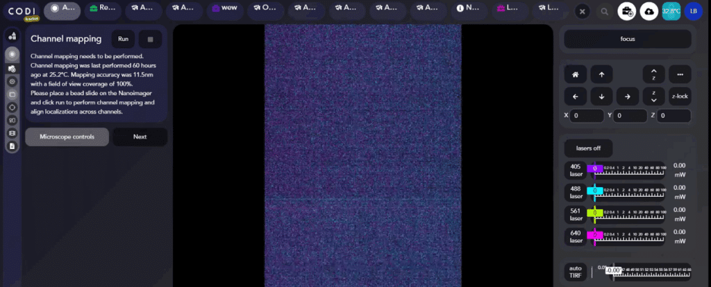
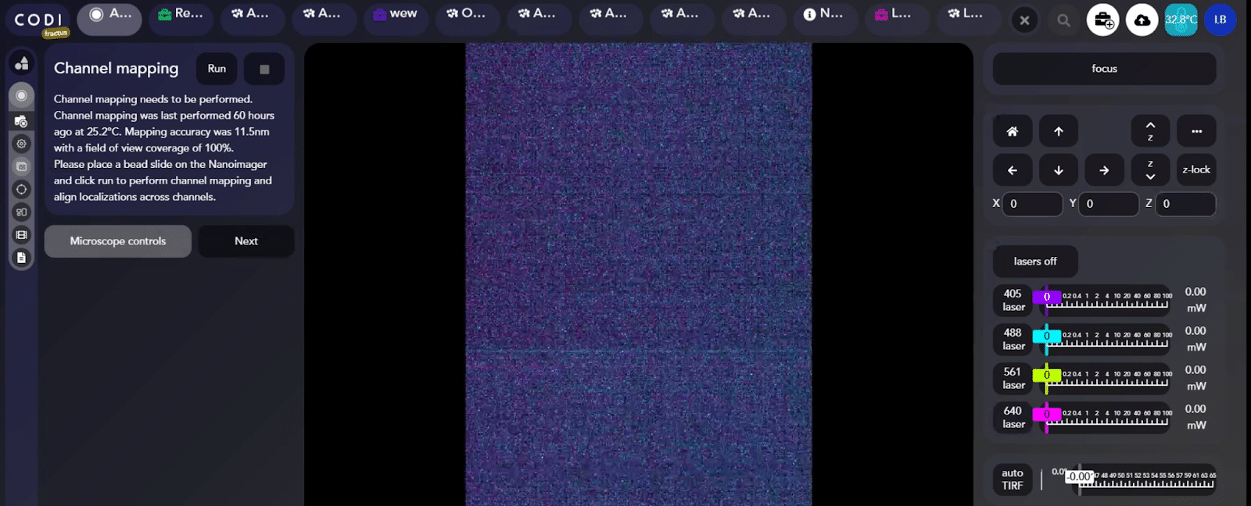
Channel mapping
Channel mapping is an essential step towards generating accurate multi-color super-resolution data, and AutoLNP makes channel mapping even easier with a one click channel mapping of both regions of the camera (left and right) that ensures PanLNP, ligand and cargo channels are mapped together.
AutoLNP simplifies your work by informing you when it’s time to run a new channel mapping or if channel mapping might need to be re-run prior to acquiring images from the LNP Profiler chip.
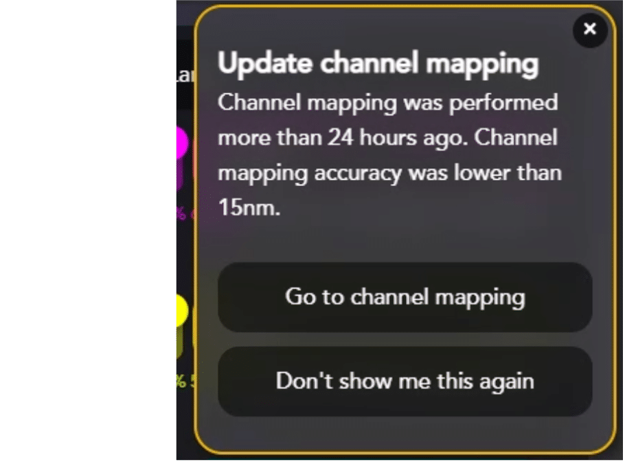
It is imperative to re-run channel mapping if:
- Channel mapping hasn’t been done in the last 24 hours
- The Nanoimager temperature has changed by >1°C since the last channel mapping
- It is the first time running AutoLNP

To run channel mapping, ensure that the bead slide is in the chip holder on the Nanoimager stage and click the Run button at the top to automatically run channel mapping. Follow the progress of channel mapping thanks to a progress bar and see each step that has been run.
Stop channel mapping at any time by pressing the ◽️ button.

Channel mapping works by first finding focus automatically using the 638 nm laser with 673/35 filter.
AutoLNP will report back the accuracy and field of view coverage of the channel mapping. An accuracy of less than 15 nm and a field coverage of 100% are recommended. Details on how channel mapping works are in Appendix 2 of this guide.
Key Tip
Channel mapping is a fairly quick process, usually taking 2 minutes. If channel mapping is taking longer, the bead slide might have a sparse bead density, which requires more fields of view and more time. If channel mapping is not complete after several minutes, stop it and replace the bead slide.
If the accuracy is less than 15 nm and/or the coverage less than 100%:
- Clean your bead slide
- Replace the oil on the objective
- Click the Re-run button to re-run channel mapping until you are satisfied.
- Click the Microscope controls button to manually diagnose sample-related issues in situations when the bead slide is not optimal or the autofocus isn’t working properly, and to display advanced microscope controls on the channel mapping page. This will help you manually jump in and diagnose sample-related issues in situations when your bead slide is not optimal or the autofocus isn’t working properly.
Channel mapping not required
While running channel mapping before the experiment is recommended, if it has been performed recently and that the Nanoimager temperature is stable, AutoLNP will allow imaging without performing channel mapping, for instance, when imaging more than one chip at once.
Calibration & sample check
For AutoLNP to be successful at imaging of LNP Profiler Assay Chip, it is essential to ensure that the chip is ready to image prior to starting the super-resolution acquisition.
Key Tip
Anytime the LNP Profiler Assay Chip is placed on Nanoimager, the system calibration step should be performed to ensure optimal autofocus and AutoTIRF.
System calibration
System calibration is a critical step that automatically finds the imaging surface of the LNP Profiler Assay Chip, locks the focus, and determines the optimal illumination angle with AutoTIRF.
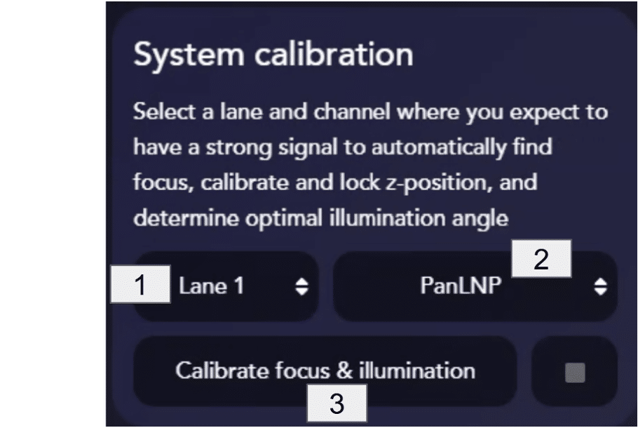
Start calibration by selecting a lane [1] and channel [2] expected to have a good LNP density and a strong fluorescent signal. For example, for LNPs labeled with PanLNP in lane 1, select that lane and then select the PanLNP channel.
When ready, click the Calibrate focus & illumination button [3] to start the calibration. Do not run the calibration in a negative control lane.

Calibration can take around 2 minutes to complete. If the wrong lane or channel is selected for calibration, this can be stopped using the ◽️ button at any time.
Calibration may fail for several reasons. Errors will appear in the top right corner indicating the reason. Common sources of failure are: inability to find the lane surface or inability to find the optimal focus based on the fluorescence signal due to too few points being detected.
- First, ensure the Assay Chip is properly positioned on the Nanoimager stage, and that the lanes are bubble free.
Note: If the failure appears to be focus related, select the Refresh z-lock calibration option.
- Try a different channel or lane where a strong signal is expected and then re-run the calibration by clicking Calibration failed. Re-calibrate focus & illumination.
- If the chip lanes are full of bubbles, proceed to prepare a new one.
- Once sample calibration has been successfully completed, the widget will update to display the calibrated focal plane and TIRF angle (bottom right). Use sample pre-check to assess the TIRF angle and modify it if needed (see details below).
Key Tip
The TIRF angle is typically between 52° and 54° on the Nanoimager and should not deviate by more than 0.5° between acquisitions.
Acquisition settings widget
Autofocus and AutoTIRF commands might not give the optimal value or even fail due to the low signal in the sample. This is why it is very important to run the Sample check.

Sample check
Sample pre-check is a great tool that quickly scans each lane of the Assay Chip and provides a representative image of the sample in each lane. It is recommended to use it for each Assay Chip to get an overview of the sample prior to imaging. This will help confirm correct sample calibration, focus and illumination; and if LNP densities are as expected, LNPs were correctly stained, and samples properly washed.

Note
The sample pre-check uses the laser powers and illumination angle from the experiment settings page, sample blinking may be observed. Laser powers can be modified for refined focus as explained in the next steps.
Click Start sample pre-check to begin the sample check, and AutoLNP will start scanning each lane.
Key Tip
The sample pre-check is intended to give a representative image of the automated acquisition, and thus uses the imaging settings (laser power and TIRF angle) from the experiment settings page.
Focus check
The autofocus tool is an automatic function to find optimal sample focus in cases where the FOV has good a Signal to Noise ratio (SNR) and there are at least 3 objects (such as LNPs or beads) when calibration is performed. Autofocus may fail or look poor if there are bubbles, low/no signal, etc.
TIRF angle check
AutoTIRF is an automatic function that finds the optimal angle for which the SNR is reduced. If the signal and the surrounding background change from sample to sample or lane to lane the AutoTIRF might output different values after every run. This is because it is calculated based on the SNR of the FOV selected during the system calibration step.
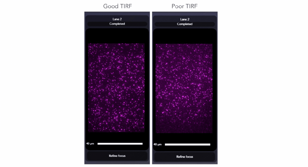
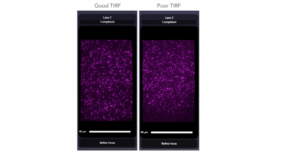
An optimal TIRF angle is required to achieve accurate quantitation. Manually inspect each lane for poor TIRF alignment. This will be visible in all lanes. A good TIRF angle will result in an even FOV illumination, low background noise, and high signal from the particles. A poor TIRF angle will result in a lack of signal in the bottom or top of the field of view. If the TIRF angle in the sample check is poor, proceed to the optimizing and setting the TIRF manually.
Optimal Focus and TIRF
If autofocus consistently fails or if autoTIRF looks poor, follow these instructions:

-
- Go to channel mapping (in AutoLNP).
- Click “Microscope controls”, the stage, lasers and TIRF widgets will appear on the right.
- Using the stage control, go to a lane where the sample is labeled.
- Switch on the 640 laser to image PanLNP and set its power at 40% as a start.
- Move the Z position until the LNPs signal comes into focus. Adjust the laser power if it is too high (bleaching fast) or too low (sample signal is dim).
- Note down the Z value and the laser power.
- Find the optimal TIRF: change the TIRF value manually until the best SNR signal is observed (bright spots, dark background).
- Go to the System Info App.
- Add the Z focus value in the acquisition settings widget. Type the value in the “Starting focus Z-position for system calibration (ONI 4-Lane Assay Chip)”, if optimizing the 4-lane chip focus.
- Click the Auto button to switch to a manual TIRF angle. Proceed to type the optimal value found manually.
- Change the optimal laser power found manually.
- Click Save Settings.
Settings can be reset to default when needed.
Refine focus in the Sample pre-check
Sometimes focus found during System calibration might not be optimal, and refining focus might be needed.
In the sample pre-check step, select Check Focus in the lane title if AutoLNP thinks manual refinement is needed, or Completed if the focus is good. If Check Focus is displayed, select the Refine Focus button.

Once Refine Focus is pressed, the Nanoimager will move to that lane, turn on the lasers, and allow the user to manually refine the focus. This is great for optimizing the focus in the rare case the sample is slightly out of focus.
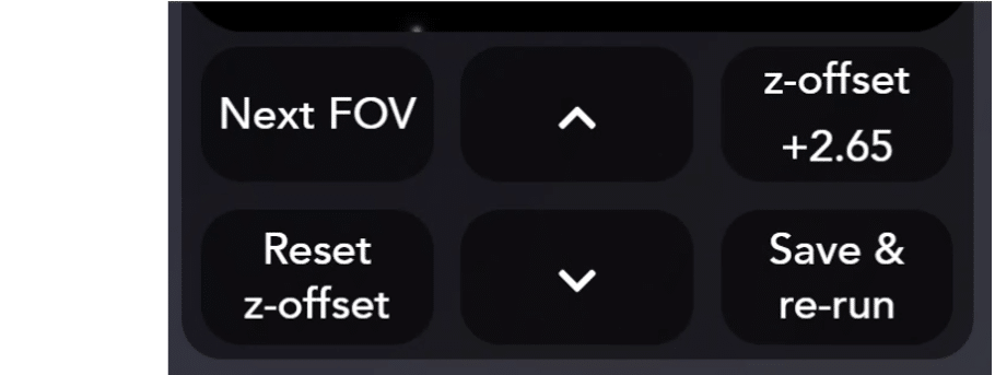
Use the “up” and “down” arrows to move the Z-offset and find the optimal focus. Click the “Next FOV” button to move to the next FOV in that lane and get a view of the focus without bleaching the sample.
When ready, click the Save & Re-run button to save the optimal focus and acquire a new sample check image.
Key Tip
Any offset applied is lane-specific and is used during image acquisition of that lane to ensure it images the best focal plane found. These settings are stored in the local storage of the web browser, and will reset to defaults if a different browser is used or browser caches are deleted. Double check these values prior to running any experiment.
Field of View (FOV) selection

In this section FOVs will be selected for image acquisition in each lane of the chip. Click the Select 6 default FOVs per lane button (top left) once to automatically select 6 default FOVs in all lanes. These are chosen to provide a good statistical distribution of LNPs. The image above shows the default 6 FOVs, optimal for most experiments as they are centered in the sample lanes and are evenly distributed.
To select different FOVs, or if the lane has a specific fault in these areas (bubbles, drying out, etc), FOVs can be manually selected. Go to the “Choose FOVs” page for that.
White vertical and horizontal lines indicate the middle and center of each lane.
Multiple FOVs can be selected per lane, 6 is the recommended number.
The selected FOVs will appear in violet.
Each time a new FOV is added, the ETA (estimated time) at the bottom left of the page is updated with the new estimated experiment duration time.
The legend shows different possible FOV status:
- A FOV previously imaged in system calibration or sample check appears in gray.
- A FOV failed to be imaged because of focus appears in red.
- The current stage position appears in blue.
- A FOV imaged during the current experiment appears in green.
Note
The FOV in AutoLNP covers an area of 50 µm (width) by 80 µm (length). Each FOV’s imaging area is surrounded by a bleaching safe zone, so that any acquisitions in the neighboring FOV will not be affected by stray laser light. The result is that each FOV rectangle in the FOV selector represents this bleaching safe area of 90 µm x 110 µm.
There are 2 other options on this screen:
- Acquire diffraction-limited image prior to super-resolution image: this acquires a single frame of each channel prior to starting the single-molecule imaging, which can be overlayed in CODI. This is great for showing the power of super-resolution images on the LNP samples (before and after!)
- Save TIFF images to disk: unchecking this box will only save the localization data to disk, saving precious disk space for long LNP acquisitions.
Each FOV corresponds to a single dataset. Multiple datasets within the same lane can be generated by acquiring multiple FOVs. Six FOVs per lane should provide a good statistical power.
Acquisition

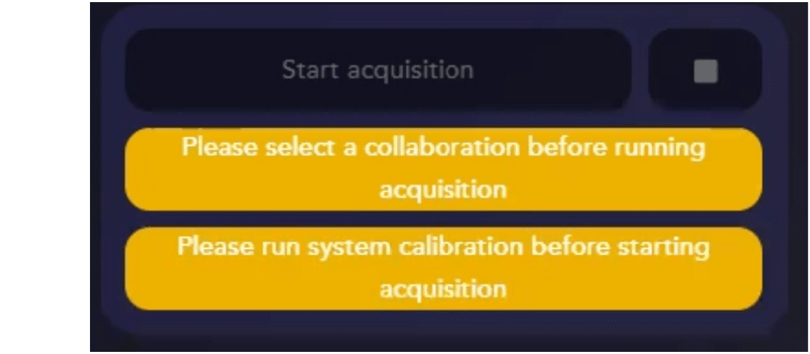
Before starting an acquisition
While many of the AutoLNP steps workflow are optional (like Channel Mapping and Sample Check), there are 2 critical steps that must be completed prior to starting the super-resolution imaging:
- Selecting a Collaboration on CODI in which to store the data and analyses.
- Running a system calibration to ensure correct focus and illumination during the acquisition.
AutoLNP will show a warning if either of these conditions are not met. The yellow warning on the banner can be clicked to explore the step to be fixed.

Starting an AutoLNP acquisition
Now that the AutoLNP acquisition is set up, click the Start AutoLNP acquisition [1]. The LNP Profiler chip will be scanned from Lane 1 to Lane 4, and the acquisition in each lane will follow the settings input in the Experiment Setup page.
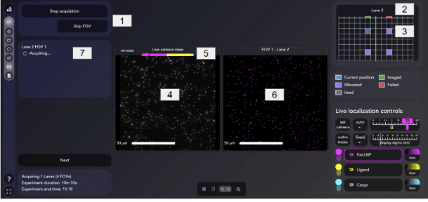
During the acquisition, real-time information shows:
- Which lane [2] and FOV [3] are currently being imaged, allocated or failed
- A live camera view [4] to see the blinking fluorophores
- A live progress bar [5] reporting frames count and estimated time of completion
- Live localizations displayed [6] from the blinking fluorophores
- A list of acquired FOVs and their status [7]
- Acquiring: The FOV is currently being imaged
- Uploading: The FOV has completed imaging and is being uploaded to CODI
- Analyzing: The FOV is being analyzed on CODI
# Clusters: The FOV is done being analyzed and is displaying the number of clusters found in the FOV
At any point during the acquisition, the ◽️ button [1] can be pressed to interrupt the acquisition, while Skip FOV button can skip the acquisition of the current FOV being imaged. If a FOV is skipped, it will not be saved nor analysed.
Each dataset will be automatically uploaded to CODI once acquired. Click any dataset from the acquisition list [7] in the acquisition page to visually inspect the sample.
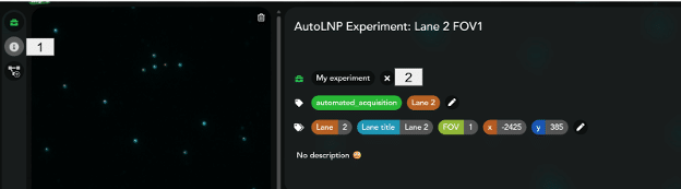
Dataset info page
After acquisition, the app will automatically open the dataset within CODI analysis. The dataset info page contains all the information about the dataset, including:
[1] Channels acquired: Cargo in DL, PanLNP and Ligand in SMLM with number of localizations displayed
[2] Focus value
[3] Z-offset
[4] Pixel size
[5] TIRF angle
[6] Stop analysis button

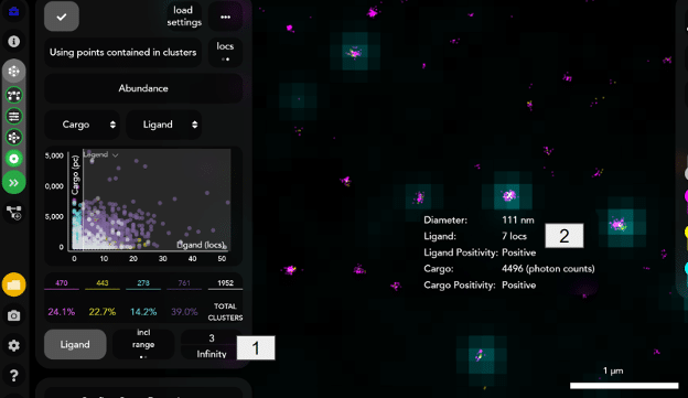
Summary & Report
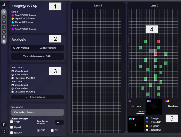
The summary page provides a quick, visual overview of the experimental results:
- Imaging Setup [1] gives an overview of the sample and imaging settings
- Analysis [2] displays the analysis settings that were used and a link to view the data on CODI
- Acquisition List [3] shows a list of all the imaged FOVs, with a link to the dataset and analysis on CODI.
- When the analysis completes, the number of clusters will also be displayed here, making it easy to see if the data had a consistent LNP density (recommended value 1500) or if some FOVs or lanes did not have a good capture.
- If an FOV failed to image (likely due to inability to properly find focus), it will not display in this list.
- Visual Experiment Overview [4] displays each FOV that was imaged for calibration, sample check, or during the super-resolution acquisition.
- Mosaic View [5] shows a representative image of each positivity class, providing a quick glance at the LNP sample. Hovering over each image allows users to cycle through more LNPs of each type and copy the image for quick sharing in a presentation.
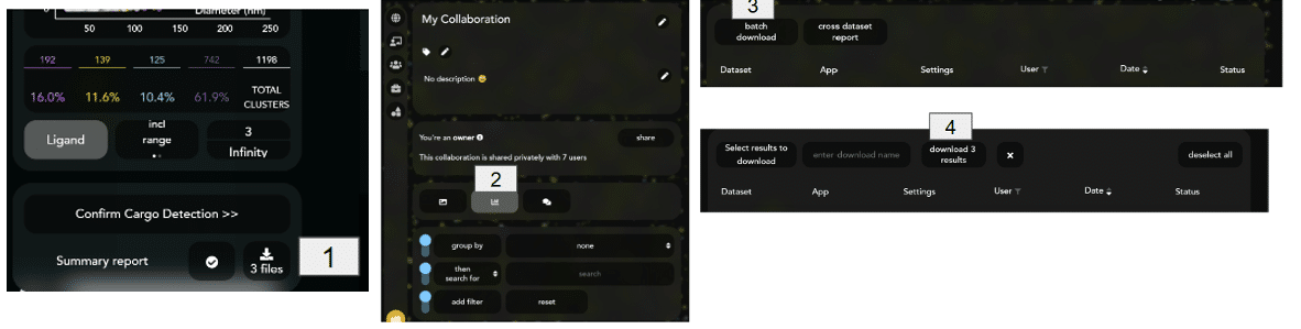
Exporting acquisition data
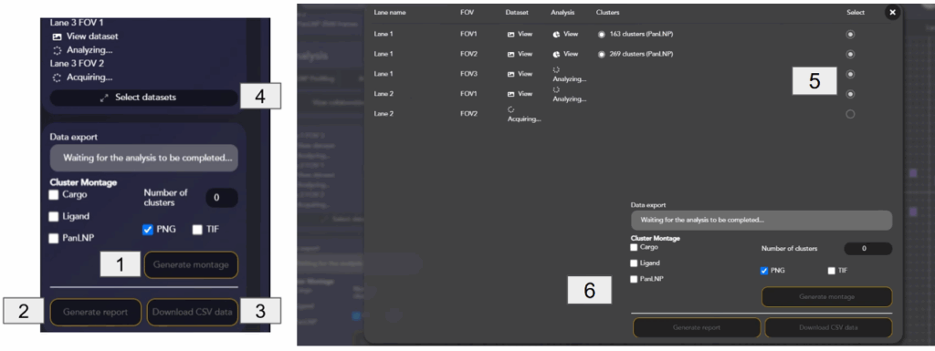
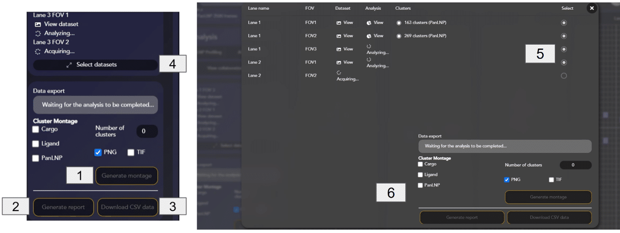
When the data is done acquiring, uploading and analyzing, it can be exported by:
- Generating a Montage of LNP clusters per chip-lane. The montage contains a visual overview of the LNP sample [1]
- Generating a Report that contains an overview of the chip’s LNP count and positivity, by lane [2]
- Downloading CSV Data that contains all the clustering and positivity data [3]
A montage, report and CSV data can be generated even if a subset of datasets is acquired, or if the analysis of some of the datasets is not yet completed or failed by clicking Select datasets [4]. Select only the datasets for which the analysis is completed [5], and use the Data export widget [6] to generate the files.
Generating a montage
Generate a montage to visually inspect the size and morphology of the LNP sample and the analysis outcome.
This feature allows the creation and saving of a montage of random LNPs selected and ordered based on positivity and size (see image below). This feature is particularly useful not only to visualize the positivity results but also to assess assay quality.

At the end of an acquisition, a montage from the 4-lanes chip or a montage from individual FOVs can be generated.
Key Tip
Once new data is acquired it will not be possible to generate a montage image for the entire chip. Ensure a montage is generated at the end of the acquisition, before moving on to the next chip. It is always possible, on the other hand, to generate a FOV montage.
How to Generate a Montage from the 4-Lane Chip
- In the summary page of the AutoLNP app, go to the “Data Export” widget and select the channels to visualize in the montage.
- Select the number of clusters per positivity group (e.g. a montage generated with 10 clusters means 10 clusters per each positivity group present).
- Select the output file format. E.g. TIFF format will allow brightness adjustment of the diffraction-limited channel using ImageJ.
- Click “Generate montage”. Note: for 4-lane montages with 50 clusters each, generating a montage requires around 15 minutes.

- A montage for each lane will be saved locally in the experiment folder under the
C:/Data/CODIpath. - Each lane montage will contain clusters coming from the FOVs acquired in that lane.
- Error messages may appear if:
- There are no clusters (analysis failed or still ongoing)
- Some lanes are missing clusters
- To generate a montage with different clusters, click “Generate montage” again. Random clusters will be selected every time.
Generate a Montage from a Single Dataset
- Navigate to one of the CODI datasets acquired with AutoLNP.
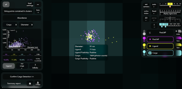
- Go to the positivity step.
- Select Confirm cargo detection [1].
- Select the number of clusters per positivity group [2]. For a single dataset and 50 clusters per positivity group, this should take about 2 minutes.
- Select the output file format [2].
- Click Generate montage.
- A montage preview will appear. To generate a montage with new random clusters, click Generate montage again.
- Downloading the montage [3] will automatically save it in the computer’s Downloads folder.


Generating a report
The report provides quantitative information on the samples to the user. Click the Generate Report button to create a report including a sample overview, the experiment performed, and the sample outcome with the imaging settings used. The report also contains the experiment title, analysis performed, date and name of the user.
The report consists of two pages. In page 1, the report outputs the LNP counts per lane and per single FOV, the overall LNP size distribution per lane, and a table with LNP size insights and Polydispersity Index (PDI). Finally, the biomarkers positivity averaged across the FOVs acquired are displayed per lane. Page 2 provides the LNP size distribution across all FOVs in a lane as a function of positivity, the LNP size distribution as a function of cargo loading, and the relative cargo abundance (in photon count) against ligand abundance (as localizations per single LNP), including a threshold red line for ligand positivity.
To print or save the report use the button. A link to the report on CODI can be saved by copying or favoriting the URL directly.
Download CSV readout
At the end of an analysis, download the csv data with all LNP outputs from the analysis. These files can be used for additional analysis and plots outside CODI.
This can be done in the AutoLNP app, under the Summary Page by clicking the Download csv data button, but also in the CODI analysis space within a single dataset in batch analysis.
When downloading the report from the Summary Page in the AutoLNP app, two zip files will be saved in the local computer’s download folder:
- “Experiment data”, includes all the raw positivity results and clustering results with csv format.
- “Experiment points data”, where a list can be found of all raw localizations before analysis tools are applied.
Important
The most important csv file will be results.csv in the Experiment data folder. This consists of a list of LNPs clustered with their given ID, centroids, area, diameter, positivity values, abundance, and discarded LNPs with the reason for discarding.
Re-running the chip
Once the summary of the acquisition is viewed and the report generated, more data from the same chip may be acquired. AutoLNP makes this really easy with the Re-Run button, which shows the experiment info page, where the number of FOVs per lane can be increased/decreased, or acquisition settings changed.
Note
If re-running a chip with more FOVs, the FOV annotation will start again from 1. Changing the experiment title is recommended, for example, adding “run 2”, so that FOVs acquired in each run can be distinguished, e.g., FOV 1 acquired during the first run and FOV 1 acquired in the second run.
Run next chip
Remove the chip carefully and place the next one. Close the LNP experiment tab and open a new one from the Acquisition apps. Load the saved experiment setting with the correct laser power that was optimized for the Nanoimager. All the next steps will be identical to the above. Only run channel mapping again if prompted by the system.
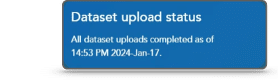
Dataset upload status
To obtain insights into the LNP sample, data acquired on AutoLNP has to be analyzed on ONI’s cloud-based software, CODI. The raw imaging data is first saved locally on the C drive on the Nanoimager laptop and is then uploaded to CODI. Upload is automatic, but it requires a stable internet connection and for CSA to be open.
Since AutoLNP is a CSA app, uploading to CODI will commence immediately after data acquisition, as long as the laptop is connected to the internet. If upload is not completed, it will begin automatically next time the AutoLNP is opened on CSA as long as an internet connection is available. In the Nanoimager App, the dataset upload status widget displays information about the upload progress. This widget will show how many datasets are in the upload queue, as well as important information if that queue is stalled, for example, if the internet connection is unreliable or unavailable.
Key Tip
The CODI System App must be open for uploads to succeed. If stalled, and the internet connection is stable, closing and re-opening the CODI System App to re-initiate the upload queue is recommended.
Batch Report
If the LNP report was not generated at the end of an acquisition in the AutoLNP app (summary page), it can be done at any time in CODI using the “Batch Report” feature, which provides a report for a single chip with up to 4 lanes. To do that, navigate to the CODI collaboration in which the data is saved and perform the following:
- Click the Analysis Results button to view all the analysis results in this collaboration.
- Click on the Cross Dataset Report button.
- Select the AI LNP Profiling analysis App, and the latest version of the settings used during the acquisition.
- Select the datasets from one chip (one dataset corresponds to one FOV) you want to appear in the report and click Generate Report.
Note
The LNP batch report is for a single chip and up to 4 lanes, i.e., it is not possible to generate a single analysis report for datasets acquired from different chips. Additionally, CODI does not support analyses and reports across different chips. ONI can provide an offline python-based code tool to generate cross-chips reports (oni.bio/contact). AI LNP Profiling can only analyze data acquired using the AutoLNP app. Data acquired using other tools, e.g., NimOS, cannot be analysed using the AI LNP Profiling, and reports will not be generated.

Troubleshooting
Dark camera streaming
If the camera stream becomes dark, in most cases, this means that the visualization has become dark, but the camera is still recording and, thus, the data is still preserved. The following can be done to restore the camera view:
- Refresh URL webpage
- Change acquisition page: go to channel mapping and come back to the acquisition page.
When following these steps, the AutoLNP CODI data will not be lost.
Sample not illuminated after opening the lid
If the Aplo Scope lid is opened while lasers are on, the interlock mechanism will be activated. The interlock mechanism makes sure the lasers are switched off automatically. When the lid is closed, the lasers will be still off, even though from the microscope control laser widget the UI will show them as turned on. The following can be done to trigger back the lasers: switch them off and on again using the microscope controls.
CODI is slow
If CODI is slow, check the following:
- Your disk memory. Make sure it’s not full
- Your Google Chrome Graphic Settings: Go to Chrome settings > System > then disable “Use graphics acceleration when available”
Help and Support
If at any time you experience a software issue, contact ONI through the Help Center (oni.bio/contact). Click on the question mark displayed in AutoLNP and CODI and go to “report an issue”.

Appendix 1 – Laser power percent to mW conversion using NimOS
Laser power percent to mW conversion using the microscope control
On Nanoimagers manufactured after January 2021, the conversion of Laser power percent to mW is accurate as long as up-to-date maintenance is performed by an ONI technician. If needed, contact ONI support for further questions.
- Go to channel mapping page
- Click “Microscope controls”
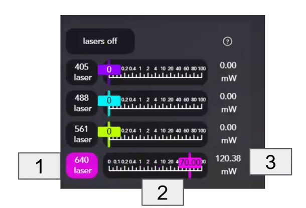
- Turn on one laser at the time [1]:
- Using the slider [2], change the power percentage value until it reaches the desired mW power [3]. Specific percentage values can also be typed in the box.
- Change the power in percentage in the experiment settings page.
- Repeat with all channels and powers indicated in the table below. Use the table to record the values for the
Nanoimager
system in use. - Once completed, save the current settings.
The next time the AutoLNP is run, go to “Load Settings” in the Experiment settings page and select the settings saved. This operation needs to be done for every user account that will use the AutoLNP, and repeated once a month to ensure that mW power and % values are always calibrated in the case the laser specs drop.
Table for recording mW to % conversion
| Laser line (nm) | Power (mW) | Power (%) | |||
|---|---|---|---|---|---|
| 640 | 60 | ||||
| 561 | 100 | ||||
| 488 | 0.15 |
Appendix 2 – Guide to AI LNP Profiling
Channel Mapping Procedure
The camera of the Nanoimager is split in two regions (left and right). Depending on the configuration of the Nanoimager being used, channel signal will be sent to the left camera region, or the right region (like for the 488 channel). AI LNP Profiling analysis makes sure that all channels are mapped correctly to each other before being uploaded to CODI. Channel mapping is used to allow the correction of chromatic aberration that results in image distortion. Specifically, the localizations in the 640 and 561 channels are mapped up to the right camera region where the diffraction-limited image is acquired such that they overlap. The mapping correction file comes from the channel mapping calibration done with beads prior to the experiment, which is why this step is such a crucial step.

AI LNP Profiling analysis
The AI LNP Profiling analysis is an automated, step-by-step, analysis workflow for LNP characterization, consisting of LNP counts, size and morphology and PDI. For each single LNP the information on cargo loading and ligand positivity and abundance can be obtained.
The workflow consists of four steps: Drift correction, Filtering, machine learning (ML)-based clustering tool, AI based Counting and Abundance tool.
The entire analysis takes 5 minutes per single dataset.
Drift correction
AutoLNP app allows users to sequentially image PanLNP, followed by Ligand and Cargo, for a total of 2 minutes per single field of view. During this time, the sample can drift in the order of a few tens of nanometers due to temperature change or physical sample movement. ONI’s drift correction algorithm allows correction for this.
Drift Correction Procedure
A standard Drift Correction at Minimum Entropy (DME) algorithm is applied to both the PanLNP and Ligand localizations, with the last frame used as reference (see CODI user guide). The diffraction-limited channel does not have drift correction applied to it. This is because the duration of that acquisition segment happens immediately after the ligand channel and only lasts briefly, so any minimal drift has negligible effect on the appearance of diffraction-limited spots.
Filtering
Each SMLM localization (namely, PanLNP and ligand channels) is characterized by sigma, precision and p-value. Minimum and maximum thresholds for these characteristics were optimized based on positive controls and negative controls. AI LNP Profiling automatically filters out localizations that don’t meet these optimized thresholds as they are identified as noise.
ML based clustering tool
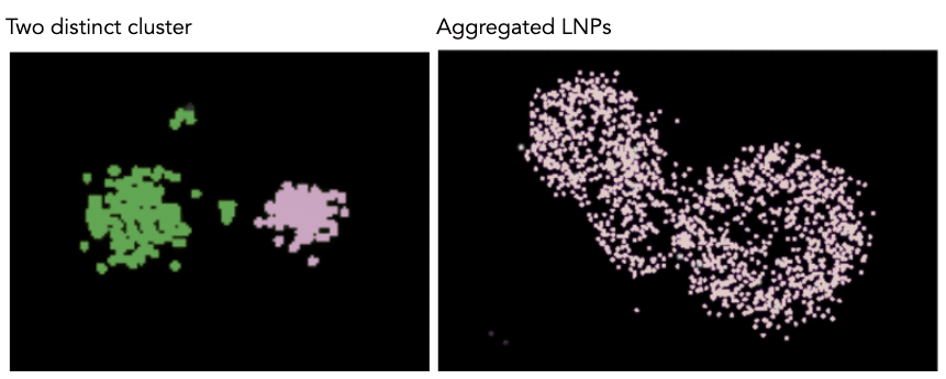
Clustering is applied to identify small and large LNPs, as well as single LNPs and aggregates. The clustering is performed exclusively on the PanLNP channel as the marker for LNP recognition.
LNPs are detected and segmented using an AI-based model, specifically a neural network vision model. Unlike algorithms like DBSCAN, which requires users to input multiple parameters, this is a one-click model with no parameters to fine-tune. Additional advantages of this model include:
- Flexibility: in accommodating different LNPs formulations, size and morphology
- Speed: fast time from acquisition to answer

Once the ML clustering model has detected LNPs (called masks), a post processing analytical step is applied to ensure that “close but separate” LNPs are identified as distinct clusters while aggregates are considered one single cluster. Once clusters are detected, any object that has less than 30 PanLNP localizations and a diameter that is less than 25 nm will be discarded as considered background noise. These filters can be changed by going to the back of the clustering widget (three dots, top right). The ML model was trained using a combination of simulated data and real acquired LNP data with a variety of background noise levels.
The model was validated over multiple independent LNP datasets to confirm that:
- it detects more than 95% of clusters, both large (up to 2 µm) and small
- it clusters single LNPs and aggregates with a 90% accuracy
The clustering tool has a run time of approximately 2 minutes for a 50 µm x 80 µm FOV.
Model output
The clustering tool segments localizations into clusters [1] and noise [2]. The segmentation is displayed to the user via colour coded points in CODI. The properties of the identified clusters including size, number of localizations, and geometry are recorded, displayed in the single cluster widget [4] and as a population level summary in the AI LNP Profiler workflow widget [3].

Note
The diameter [4] is based on the calculation of a circle with the convex hull area extracted from a single LNP. The formula for PDI [3] is (SD/Mean)2, where SD and Mean refer to the size distribution in the sample.

It is possible to select and identify clusters by their ID. To do so, visit the back of the widget [5], where more information is displayed. To be specific:

- Selected cluster ID: the ID of the currently selected cluster in the CODI dataset. The same ID will be found in the cluster CSV file.
- Download clusters CSV button: Users can download the properties of all clusters detected as CSV file by clicking Download csv data. The file will be downloaded to the Downloads folder. This file contains the list of all the clusters with properties associated with them. Specifically: Cluster ID, X, Y, Number of localizations, Skew, Circularity, Density, Area, Discretized area, Radius of gyration, Length, Diameter.
Additional information includes:
- Channels to cluster on
- Clustering model version
- Minimum localizations and minimum diameter thresholds per LNP, applied after the clustering tool is run to remove all clusters that have less than a given number of localizations and a size smaller than a given value.
Key Tip
Leaving all the parameters to the default ones is recommended as these are the optimal for the LNP kit.
AI based Counting and Abundance tool
After clustering is completed, a two-steps positivity and abundance tool is run:
- AI unsupervised model for cargo detection
- A count–based method for ligand detection and abundance
The cargo positivity tool is based on a machine learning model that detects if a single LNP has cargo, based on its image properties compared to the local intensity background. Cargo abundance refers to the overall intensity in photon counts of the given LNP with the local background subtracted.
The positivity tool starts by averaging all the cargo frames acquired into a single 2D image to represent the overall signal. Camera calibration is applied to the final image to correct for pixel sensitivity variations and to remove hot pixels, converting the signal into photon counts. Next, a background correction algorithm is applied to the image where no cargo signal associated with an LNP is present.
A machine learning model is run to determine whether each individual LNP contains cargo. In the final output, all LNPs will be defined either as cargo negative or positive. The cargo positivity model has an accuracy of 90%. There are two machine learning models: v1 (legacy) and v2 (recommended / default).
AI LNP Profiling v1 (GMM Model) – legacy
The AI LNP Profiling V1 uses an unsupervised Gaussian Mixture Model (GMM) to determine cargo positivity using hand-crafted image metrics extracted from cargo-channel patches around each Pan-LNP cluster. This model has a 90% accuracy performance when a single LNP cluster has no cargo signal in the nearby proximity.
AI LNP Profiling v2 (CNN Model) – recommended / default
The AI LNP Profiling v2 uses a Convolutional Neural Network (CNN) to classify cargo positivity from cargo-channel patches centred on each Pan-LNP cluster centroid. The CNN is a supervised, patch-based classifier that learns visual features directly from the cargo channel rather than using hand-crafted metrics. It outputs a binary cargo-positive / cargo-negative prediction for each detected Pan-LNP cluster with an accuracy of 90%. It is set as the default in the AutoLNP app and improves performance (notably reducing false negatives) versus v1, particularly when the LNP density is high in a FOV, allowing classification of each LNP in the proximity of a cargo spot. In the figure, an example of clusters classified positive (1) and negative (0) by the CNN and GMM models are displayed.

Relative cargo abundance computation
To determine the cargo abundance coming from the diffraction limited cargo signal, an artificial region around each LNP cluster, whose size is derived from the Point Spread Function (PSF) of the cargo channel, is drawn. Relative cargo abundance is calculated as the sum of all cargo photon count inside the artificial region.
Important
Due to the local background subtraction mentioned above, only relative abundance values can be reported. These values do not correlate with single cargo quantification.


Discarded LNPs
LNPs showing certain characteristics related to the diffraction-limited channel will be discarded from the positivity analysis. The reason is that the cargo positivity might be compromised and therefore these LNPs are automatically rejected. All LNPs remain available in the CSV covering the full results, but they are not included in the summary statistics of the positivity phenotype breakdown. There are three cases for discarded LNPs:
- Background instability: this is the case where there is an extremely bright cargo spot near an LNP. Its presence will impact the background subtraction step and the overall cargo signal readout.
- Proximity*: the cargo positivity tool cannot predict in advance if an LNP has true cargo or not, therefore if two clusters or more are “too close” in the PanLNP channel they will be discarded from the positivity analysis, regardless of the cargo signal presence. This is because the cargo PSF coming from each LNP may overlap and lead to difficulties in classifying their positivity and measuring their abundance.
- Edge proximity: if an LNP is located near the borders of the field of view it can lead to inconsistencies in patch size, which can lead to aberrant effects in the positivity classification. This proximity is set to 5 pixels from the edge of the field of view: if all localizations of a given LNP are within that range, they will be discarded.


For each of these cases, the abundance is set to 0, and the CODI user interface as well as the csv output will mark these LNPs as ‘discarded’, giving the reason for the discard.


*LNP proximity
The proximity metric takes into account the effects of multiple nearby LNPs on a selected one. The procedure is as follows:
- A theoretical PSF model for the cargo channel is calculated based on information about Numerical Aperture of the microscope objective and the emission wavelength. A circle is drawn per each LNP based on the convolution of the artificial PSF with the LNP cluster area.

- For each LNP localization, the area intersected with the nearby circles is calculated: if more than 20% of the circle area intersects with nearby LNP circles, that LNP is discarded. Note that this does not automatically discard its neighbours.
Note that this discarding procedure is performed regardless of the diffraction-limited channel.
Key Tip
The number of total LNPs counted during clustering can be higher than the number of total LNPs after the positivity tool step, as LNPs will likely be discarded along the process.
Count based method for ligand detection and abundance
The ligand channel is acquired in SMLM mode, therefore, the ligand positivity tool gives information on positivity and relative abundance of the ligand based on the number of localizations counted per single LNP. Ligand localizations are detected and counted for every LNP cluster. A minimum of 3 localizations is set as a threshold for LNP ligand positivity [1], i.e., it is considered positive if it has at least 3 localizations in the ligand channel. The minimum localization value was found to be the optimal, after running negative and positive LNPs controls, and it accounts for any localization noise in the negative LNPs control. A single localization is a representation of a single fluorophore blinking event. A single fluorophore can produce multiple localizations. Additionally, more than one ligand detection molecule may bind to a single ligand on the LNP surface. Due to these factors, the number of ligand localizations is not one to one equivalent to the number of ligands present on an LNP. Trends in ligand localizations (i.e. 10 localizations vs 50) can be interpreted as a representation of the amount of ligand present on an LNP. For each LNP, the relative ligand abundance represented by the number of ligands localization as well as the positivity output is reported in the CODI user interface as well as the csv output [2].
Montage auto-brightness pre-processing
The montage tool generates downloadable PNG and PDF files that were pre-processed with auto-brightness. First, the diffraction limited (DL) image is changed from 16 to 8 bit to speed up image processing. Next, auto-brightness is applied for better, consistent visualization: specifically, the overall minimum and maximum intensity values are extracted from the entire FOV image and used to rescale the image for consistent brightness. Last, there is an extra rescale step happening both for a single montage generation or for a montage generated at the end of the acquisition across different FOVs:
- The user selects the numbers of clusters to be plotted in the montage
- The absolute minimum intensity is extracted from all selected clusters
- The following equation is applied for rescaling:
If diff (min-max) < (diff (0-255)/2), then
max = abs(min) + 255/2
CSV readout
At the end of an analysis a csv file with all the LNP outputs from the AI LNP Profiling analysis can be downloaded. This can be done in the AutoLNP app, under the Summary Page by clicking the Download csv data button, but also in the CODI analysis space within a single dataset [1] or in batch analysis [2-4].

If done from the Summary Page in AutoLNP, two zip files will be downloaded to local computer’s Downloads folder:
- “Experiment data”: contains clustering and positivity results, use this file for any post processing with external offline tools
- “Experiment points data”: contains the list of all localizations. This is more for offline advanced post processing analysis.
The most important csv file is results.csv, consisting of a list of LNPs clustered with their given ID, centroids, diameter, positivity, relative abundance, discard reasons, and extra readout such as skew, circularity, and area.
Appendix 3 – CODI: Collaborative Discovery platform
CODI is a cloud-based environment for running automated workflows (such as AutoLNP), uploading data, analyzing, sharing, and managing single-molecule localization microscopy data generated exclusively by the ONI’s microscopes. As the name indicates, CODI is designed with collaboration at its core, empowering researchers to work together seamlessly.
Creating a Collaboration
A collaboration is like a folder where a group of datasets can be stored and shared at once with colleagues. To create a collaboration:
- Navigate to the “Collaborations” tab in CODI’s main interface.
- Click on “Create New Collaboration” to start a shared workspace.
- Name the workspace and provide a brief description to specify its purpose (e.g., “LNP Profiling Project” or “Clustering Analysis Study”).
- Set permissions and roles for collaborators:
- Owner: Full control over the workspace.
- Analyst: Ability to modify and upload data.
- Viewer: Restricted to viewing.
Inviting Collaborators:
Enter the CODI account names of the team members to invite and share the link with them. Once done, the members will automatically get access to the dataset.
Adding Data to a Collaboration
- Uploading single dataset:
- Within the collaboration workspace, click “Add Data” or “Upload Dataset”.
- Drag and drop files directly, or browse to select files from the device.
- CODI supports only data format generated by ONI’s microscopes. Datasets from other microscopes are not supported on the platform.
- Uploading multiple datasets to a collaboration:
- Use the Desktop uploader software:
How to guide: The CODI Desktop Uploader
- Use the Desktop uploader software:
- Organizing Data:
- Use collaborations or tags to categorize datasets (e.g., by experiment date, project phase, or sample type).
- Add metadata to each dataset for better context. For example:
- Experiment conditions.
- Sample preparation protocols.
- Keywords for searchability.
Moving Datasets Between Collaborations in CODI
To move a dataset from one collaboration to another:
- Open the Dataset Info Page:
- Locate the dataset to be moved within its current collaboration.
- Click on the dataset to access its information page.
- Remove the Dataset from Its Current Collaboration:
- On the dataset info page [1], find the “Collaboration” section.
- Click the “X” [2] next to the current collaboration’s name to remove the dataset from that collaboration.
- Add the Dataset to a New Collaboration:
- Go to the empty collaboration where the dataset(s) is to be moved.
- Use the “add dataset” [3] feature to include the datasets directly.
- To streamline this process, consider adding a custom tag to the datasets to be moved. For instance, assign a unique tag (e.g., “ToMove”) to easily filter and identify the datasets for transfer.

Appendix 4 – Manual System Calibration
Manual System Calibration allows users to manually inspect the sample and create illumination and per-lane focus calibrations, which are required to automatically and accurately acquire FOVs across all lanes.
The Manual System Calibration page can be accessed at any time during an automated imaging workflow, and it is conveniently located before the required workflow steps.
When to use Manual System Calibration
Manual calibration can be used at any point prior to starting an automated acquisition:
- The user can opt to manually create the focus and illumination calibration instead of using the automated system calibration for a variety of reasons, including:
- Speed: once familiar with the process of creating a manual calibration, this might be quicker than running the automated calibration and sample pre-check.
- Sparse samples: for very sparse samples with <100 particles per FOV, the automated algorithms may struggle, and the user can opt to manually calibrate.
- Focus control: manual calibration allows the user to set and confirm the optimal focus per lane, ensuring data is acquired with optimal focus for all lanes.
- If an automated system calibration fails for any reason (including not enough signal detected at the autofocus position, or failure to optimize the illumination angle), the user will be prompted to create a manual calibration. In this case, the Manual System Calibration icon will be highlighted in yellow, indicating that the system is recommending the user to inspect their sample and manually calibrate.
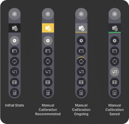
When creating a manual calibration, the user can easily follow which step of the workflow they were on by looking for the icon with an upper outline in yellow.
Once the manual calibration is saved and used for the experiment, the manual calibration page will appear with a green underline, reminding the user that they are using a manual calibration.
While the Manual System Calibration allows the user to manually find and optimize these values and save them for use during automated acquisition, the automated System Calibration step performs several automated routines to find the optimal focus and illumination angle. Read the “Creating an experiment calibration” section below for more details.
What is an Experiment Calibration
The Experiment Calibration contains information about the specific system and ONI Assay Chip to ensure focus and illumination are optimized for automated imaging:
- The stage z position where ONI 4-Lane Assay Chip is in focus, and the z-lock is set. Since the stage and the objective are not perfectly perpendicular, it is common to have a small shift in this position across lanes.
- The z-lock offset for each lane. While most chips will have the same z-offset for each lane, it is possible that certain systems or chips require a per-lane offset from the focus reference. This is the same as the z-offset set for a lane during the “refine focus” step of sample pre-check.
- The illumination angle (also called the TIRF angle) that will be used for the acquisition.
Note
The experiment calibration that is created is local to the current workflow and is not shared across different experiments. A calibration must be created for each instance of AutoLNP independently to ensure accurate automated acquisition.
Creating an Experiment Calibration

To create an experiment calibration:
- Position the stage such that a lane is over the objective
- If starting a manual calibration from scratch, note that the sample stage will be at (0,0,0), in between lanes 2 and 3. To properly focus, move to a lane where particles and a strong fluorescence signal are expected (such as a positive control lane). Choose a lane from the Experiment Calibration [1] and click the target icon [2] to move that lane.
- If starting after an incomplete automated system calibration, the sample will be positioned in the lane chosen for calibration.
- Find the focus of the particle surface
- Use “Scan for Surfaces” [3] to detect all the potential surfaces at the current (x,y) stage position. This scans the stage in the z direction and uses an internal focus camera to detect surfaces where there is a strong refractive index difference. Optionally, turn on an imaging laser [4] to observe the focus sweep on the live camera view to help see the best focus position during the scan.
- Detected surfaces appear as purple dots along the focus indicator graph
- Click on any of the detected surfaces (purple dots) to move the stage to that position
- It is common to have multiple (at least 2) surfaces from an ONI 4-Lane Assay Chip.
- Generally, the particle surface is the top-most surface.
- Turn on an imaging laser [4] to observe the fluorescence from the particles on the surface
- Refine the focus [5] until the sample is in focus. Use the Up/Down arrows in the Stage Control widget. Use the W/S keys on the keyboard.
- If necessary, move to a new FOV using the up/down/left/right FOV buttons [6]
- Calibrate the z-lock [7]
- When the sample is in focus, click the “Calibrate” button to calibrate the z-lock. This sweeps the stage in the z-direction and creates a calibration of the focus camera signal, which is used to maintain the z-position over time.
- If the calibration is successful, the z-lock will automatically engage (the lock icon will turn blue).
- Create the Experiment Calibration [8]
- Select the slide type being used for calibration. In general, this will be the LNP 4-lane Assay Chip.
- Set the illumination angle for the experiment
- With an imaging laser on, use the illumination angle slider to find the optimal angle for particle imaging. This is generally near the TIRF zone, in the 45-55° range for an Aplo Scope.
- Once the optimal angle has been determined, click the “Set TIRF angle” button to save it to the calibration
- Set the focus reference and offset for each lane
- Click on Lane 1
- Click on the target icon to move to Lane 1. While the stage is moving, the laser and z-lock are both off.
- Wait until the stage has reached Lane 1. Once the stage has arrived at its position, the laser will turn on and the z-lock will engage. This can take several seconds. Wait for the system to complete these tasks.
If the z-lock cannot be re-engaged after moving to the designated lane, an error message will appear. This is likely due to a bubble being present in the lane.
If this occurs, use the Up/Down/Left/Right FOV buttons to scan the stage until the imaging area is outside of the bubble. The best practice is to turn off the laser during this process
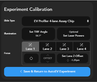
Once in a good FOV, click the lock button to re-engage the z-lock. It is OK if it is slightly out of focus.
-
-
- Use the up/down arrows in the experiment calibration widget to refine the focus until it is optimal for the designated lane.
- Click “Set Lane Z-Offset” to set the z-offset for this lane to the experiment calibration.
- Repeat this process for all lanes. Note that a z-offset must be set for each lane.
-
- Save the experiment calibration.
- Once the TIRF angle and z-offsets for each lane have been set, the “Save & Return to Experiment” button will turn blue.
- Click this button to save the calibration and use it for the active experiment.
Note
The “Save & Return to Experiment” button will be enabled once the TIRF angle and the z-offset for all 4 lanes have been set. This button must be clicked for the AutoLNP experiment to use manual calibration.
- Continue to sample check, select FOVs, and imaging
- The AutoLNP experiment will now use the values manually set during Manual System Calibration.
- The automated acquisition will now use the manually defined TIRF angle and apply the z-offset specified for each lane while imaging FOVs in the corresponding lane.
Optionally setting the laser powers for optimal blinking
In some cases, it might be necessary to manually adjust the laser powers to ensure the sample is blinking correctly. Manual System Calibration makes this process very simple:
- Once focus and TIRF angle have been optimized, turn on one of the lasers that will be used for imaging and adjust the power until optimal blinking is achieved for that fluorophore. This will depend on the fluorophore, sample type and labeling density. Contact ONI support for more information on how to determine the optimal power.
- Click the “Set laser powers” button, which will now indicate the active laser wavelength and power. This will save the currently active laser power to be used for all lanes of the current experiment.
- Repeat this for each laser that will be used for the experiment.
- When returning to the Experiment Setup page, note that the laser power for all lanes has been updated.
Optionally Setting Global System Settings [9]
Manual System Calibration can be used to set the “Acquisition Settings” from the System Info page with the correct values based on the current sample on the microscope.

Best practice for using these quick actions is (with a 4-lane Assay Chip on Aplo Scope):
- Find the focus of the selected slide type using the focus controls, and calibrating and engaging the z-lock [1]. Click “Set as initial focus for ONI 4-lane Assay Chip” to save the current stage z-position as the global default initial position when using autofocus in the system calibration, sample check and automated FOV acquisition.
- Find the lowest laser power where fluorescence with a good signal to noise can still easily be detected, and where the sample is not blinking. This may be anywhere from 3% to 25%, depending on the laser and the system. Click the “Set as laser power for calibration” to save this power as the power used for the autofocus and autoTIRF during automated system calibration.
- With the laser set to a typical power used for data acquisition (generally around 50%), use the illumination angle slider to find an angle where the sample has the highest signal to noise ratio.
- Click the “Set as manual TIRF angle” to save this as the default manual TIRF angle.
Note this does not set the system to manual TIRF mode. To do so, navigate to the system info page and swap from “auto” TIRF mode to manual.
AutoLNP for Aplo Scope
Print Section
Overview
AutoLNP is a CODI application that connects Aplo Scope to ONI’s CODI cloud-based analysis platform, enabling precise LNP characterization using the ONI Application KitTM: LNP Profiler Kit. When combined with Aplo Scope, AutoLNP uses several advanced features to provide super-resolution imaging and analysis of an entire 4-lane LNP Profiler chip with reduced hands-on time and a very robust pipeline.
Aplo Scope Requirements
AutoLNP requires active internet connection on Aplo Scope PC.
Prior to using AutoLNP
Placing the chip holder on the Aplo Scope
AutoLNP comes with a handy chip holder that makes Aplo Scope feel like it was made for LNP Profiler chips. It also allows AutoLNP to know where each lane is without any further specific calibration.
Warning
With the Aplo Scope still switched off, place the chip holder on the Aplo Scope before opening CODI System App (CSA). Make sure the chip holder lies flat.
- Place the chip holder on the Aplo Scope stage as shown in the illustration below.
- Place the LNP Profiler chip or bead slide (with magnets) inside the chip holder.
Installation & temperature setup
To run the LNP Profiler kit, you will need to register to ONI’s CODI software platform, download the CODI System App and use AutoLNP app.
Navigate to https://alto.codi.bio to access the CODI platform, and make sure to sign and log in, see [1] on the image above. If this is the first time creating an account in CODI, contact ONI to get the AutoLNP app activated. Once logged in, look for the microscope temperature control [2], and the Application apps [3] where AutoLNP can be accessed.
Go to Application apps, and select the AutoLNP app. You will see a pop up message appearing. If this is the first time you are downloading CODI System App, please click “download” as shown in the popup message and follow the instructions to install CODI System App. You may encounter “Windows Security Alert” – you must “allow access” to ensure that AutoLNP functions correctly.

Go to the Application apps, including:
- The AutoLNP app, to run LNP chips
- System Info app, to adjust system settings such as temperature or calibration power
Select the AutoLNP app. If this is the first time downloading the CODI System App, click “Download” as shown in the popup message. Follow the instructions to install the CODI System App. If a “Windows Security Alert” appears, “allow access” to ensure that AutoLNP functions correctly.
Once installed, open CODI system App and wait for the status indicator to change from “Initializing” to “Running”. CODI System App starts heating Aplo Scope as soon as the application is opened. Click the “Refresh Page” button to close the popup widget.
Key Tip: Ensure that the CODI System App is displaying “Running” prior to running AutoLNP, to ensure that Aplo Scope communicates properly with CODI.
Setting a default Aplo Scope temperature
In the top right corner of your CODI page [2], click on the temperature icon with a blue background, which will bring you to the System Status App. Here you can set your desired temperature and adjust acquisition settings. This will be saved as the default temperature for the next time you launch the CODI System App. For LNP Profiler, the default temperature is the recommended 32°C. Now, whenever you launch CODI System App, your Aplo Scope will automatically start heating to 32°C. This typically takes 60 minutes.
Key Tip
Wait 2 hours for the system temperature to stabilize before starting imaging. Any acquisition done during the heating process, will result in a lot of drift. See channel mapping section for more details.
AutoLNP acquisition app
AutoLNP is a linear workflow that helps guide users through the acquisition of the LNP Profiler kit, from experimental setup to acquisition summary. Each step of the workflow has a dedicated page, which can be accessed from the toolbar on the left hand side of CODI.
Move between the pages either by clicking on the individual tabs, or by using the action button on each page to proceed to the next step, e.g., Next, Run, Start acquisition etc.
Experimental setup
- AutoLNP experiment title (chip/sample name):
Give the experiment a name. The datasets will be saved both locally (C:/data/CODI) and on CODI using this name—pick a good one! - Dataset tags: Tags and Key/Value Tags (optional):
Add tags to help distinguish datasets on CODI. Make sure to click the Save button to save any changes. - Collaboration in CODI:
Select a collaboration in CODI where the data will be saved, or use the + button to create a new collaboration.Note: Saving to a Collaboration from AutoLNP is required. - Analysis settings:
The default “AI LNP Profiling” settings are optimized using multiple LNP types. These can be adjusted as needed to suit different analysis needs. - Experiment Settings:
Optimal experiment settings (e.g., channel names, laser powers, number of frames, and exposure times) are preselected.Note: Ensure settings are properly calibrated for each instrument by measuring laser power in mW and adjusting as needed. See Appendix 1 for details.
Data and analysis settings
AutoLNP automatically uploads the data to the selected CODI account and saves it locally in the C:/Data/CODI/ folder. The acquisition data is saved in subfolders with names corresponding to the Experiment and Lane titles provided on this screen.
Sample and acquisition settings
Setting up the acquisition to mimic the LNP Profiler Assay Chip with a 4-lane design.
- Enter a Lane Title that represents the LNP sample in that lane (e.g., LNP1 standard control, negative control, or the sample name).
- The channel name field can be edited to match a specific cargo or ligand name.
- For LNPs with both cargo and ligand, leave all channels on. If the LNP sample lacks cargo or ligand, switch that channel off using the vertical slider on the left.
- AutoLNP first acquires the PanLNP using the 638 channel in SMLM mode, then the Ligand in the 561 channel (SMLM), and finally the Cargo in the 488 channel (DL).


AutoLNP provides default starting settings recommended for running the LNP Profiler protocol. Adjust the acquisition settings by clicking on the small text below and input:
- Laser powers: prior to starting an experiment, ensure the channels have the optimized laser power to run the LNP Profiler kit. See “Optimize laser powers section”.
- AutoTIRF automatically finds the optimal illumination angle for LNP imaging by maximizing the signal to noise ratio of the spots with respect to the background. The optimal TIRF angle is determined during the “System Calibration” step, using the selected lane and channel. At any time, the TIRF angle can be manually input in the System Info app. See the “Check TIRF angle” sub-section under the “Calibration & Sample Check” section to select the optimal TIRF angle.
- Using the default settings for the number of imaging frames and the exposure duration is recommended, as they were optimized for this kit. However, these can be adjusted on a per-channel and per-lane basis if needed.
Laser power optimization
The Aplo Scope contains an internal laser power sensor, which is calibrated out of the factory to estimate the laser power at the sample. AutoLNP leverages this internal sensor to find the optimal power for the LNP Profiler Kit.
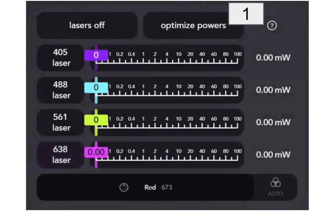
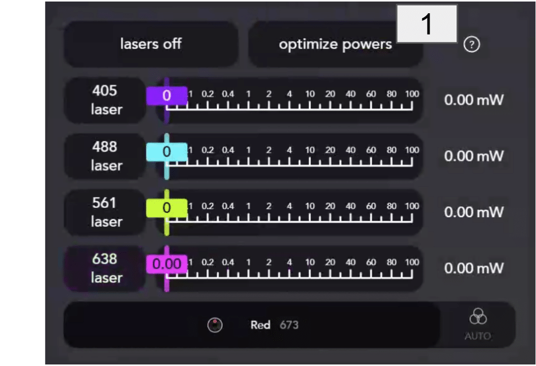
Each LNP Profiler kit needs to be acquired with a specific optimized power to ensure proper blinking of the fluorophores and the reduction of photobleaching for the diffraction–limited dye.
The Aplo Scope contains an internal laser power sensor, which is calibrated out of the factory to estimate the laser power at the sample. AutoLNP leverages this internal sensor to find the optimal power for the LNP Profiler Kit.
In the channel mapping page, click Microscope controls and then Optimize powers [1]. An automated laser power optimization routine will run, using the internal laser power sensor to automatically find the right output for each laser. This is required to achieve the adequate laser power at the sample, which may vary over time with laser output variation. This step takes less than one minute. Once completed, the laser power percentage in the experiment settings will be automatically updated for those specific experiment settings and a “Laser powers calibrated & applied to the experiment” message will appear. Values can be saved using the Save Current Settings button, and reloaded in a future experiment. The settings are saved for each CODI user.
If a particular power cannot be reached within a 10% tolerance range, AutoEV will display an error message. Should this occur, please contact the ONI Service Desk for assistance.
Key Tip
It is recommended to run the laser power optimization once a week.
Applying modified settings across all lanes
AutoLNP has a couple of options to simplify the process of applying the settings to all lanes.
Input the settings in lane 1, then use the buttons at the bottom of that lane to:
- Apply all settings: synchronize all sample and acquisition settings to all lanes
- Apply imaging settings: synchronize only the acquisition settings (channel and lane names will not be synchronized)
- Reset settings to default: reset all lanes to the default LNP Profiler Kit protocol recommendations
Save your own experiment settings
If the imaging settings are updated, such as number of frames or laser power, these can be saved by clicking Save Current Settings. These can be loaded again using Load Settings.
Note
Settings are saved locally on the Aplo Scope laptop only and NOT saved on CODI. If web browsers or users are changed, settings will need to be reentered and re-saved.
Channel mapping
Channel mapping is an essential step towards generating accurate multicolor super-resolution data, and AutoLNP makes channel mapping even easier with a one click channel mapping procedure that optimizes the PanLNP, Ligand and Cargo channels.
AutoLNP simplifies your work by informing you when it’s time to run a new channel mapping or if channel mapping might need to be re-run prior to acquiring images from the LNP Profiler chip.
It is imperative to re-run channel mapping if:
- Channel mapping hasn’t been done in the last 24 hours
- The Aplo Scope temperature has changed by >1°C since the last channel mapping
- It is the first time running AutoLNP
To run channel mapping, ensure that the bead slide is in the chip holder on the Aplo Scope stage and click the Run button at the top to automatically run channel mapping. Follow the progress of channel mapping thanks to a progress bar and see each step that has been run.
Stop channel mapping at any time by pressing the ◽️ button.
Channel mapping works by first finding focus automatically using the 638 nm laser with 673/35 filter.
AutoLNP will report back the accuracy and field of view coverage of the channel mapping. An accuracy of less than 15 nm and a field coverage of 100% are recommended. Details on how channel mapping works are in Appendix 2 of this guide.
Key Tip
Channel mapping is a fairly quick process, usually taking 2 minutes. If channel mapping is taking longer, the bead slide might have a sparse bead density, which requires more fields of view and more time. If channel mapping is not complete after several minutes, stop it and replace the bead slide.
If the accuracy is less than 15 nm and/or the coverage less than 100%:
- Clean your bead slide
- Replace the oil on the objective
- Click the Re-run button to re-run channel mapping until you are satisfied.
- Click the Microscope controls button to manually diagnose sample-related issues in situations when the bead slide is not optimal or the autofocus isn’t working properly, and to display advanced microscope controls on the channel mapping page. This will help you manually jump in and diagnose sample-related issues in situations when your bead slide is not optimal or the autofocus isn’t working properly.
Channel mapping not required
While running channel mapping before the experiment is recommended, if it has been performed recently and that the Aplo Scope temperature is stable, AutoLNP will allow imaging without performing channel mapping, for instance, when imaging more than one chip at once.
Calibration & sample check
For AutoLNP to be successful at imaging of LNP Profiler Assay Chip, it is essential to ensure that the chip is ready to image prior to starting the super-resolution acquisition.
Key Tip
Anytime the LNP Profiler Assay Chip is placed on the Aplo Scope, the system calibration step should be performed to ensure optimal autofocus and AutoTIRF.
System calibration
System calibration is a critical step that automatically finds the imaging surface of the LNP Profiler Assay Chip, locks the focus, and determines the optimal illumination angle with AutoTIRF.
Start calibration by selecting a lane [1] and channel [2] expected to have a good LNP density and a strong fluorescent signal. For example, for LNPs labeled with PanLNP in lane 1, select that lane and then select the PanLNP channel.
When ready, click the Calibrate focus & illumination button [3] to start the calibration. Do not run the calibration in a negative control lane.
Calibration can take around 2 minutes to complete. If the wrong lane or channel is selected for calibration, this can be stopped using the ◽️ button at any time.
Calibration may fail for several reasons. Errors will appear in the top right corner indicating the reason. Common sources of failure are: inability to find the lane surface or inability to find the optimal focus based on the fluorescence signal due to too few points being detected.
- First, ensure the Assay Chip is properly positioned on the Aplo Scope stage, and that the lanes are bubble free.
Note: If the failure appears to be focus related, select the Refresh z-lock calibration option.
- Try a different channel or lane where a strong signal is expected and then re-run the calibration by clicking Calibration failed. Re-calibrate focus & illumination.
- If the chip lanes are full of bubbles, proceed to prepare a new one.
Key Tip
The TIRF angle is typically between 54° and 60° on the Aplo Scope.
Acquisition settings widget
Autofocus and AutoTIRF commands might not give the optimal value or even fail due to the low signal in the sample. This is why it is very important to run the Sample check.
Sample check
Sample pre-check is a great tool that quickly scans each Assay Chip lane and provides a representative image of the sample. It is recommended to use it for each Assay Chip to get an overview of the sample prior to imaging. This will help confirm correct sample calibration, focus and illumination; and if LNP densities are as expected, LNPs were correctly stained, and samples properly washed.
Key Tip
The sample pre-check is intended to give a representative image of the automated acquisition, and thus uses the imaging settings (laser power and TIRF angle) from the experiment settings page.
Click Start sample pre-check to begin the sample check, and AutoLNP will start scanning each lane.
Key TIp
The sample pre-check is intended to give a representative image of the automated acquisition, and thus uses the imaging settings (laser power and TIRF angle) from the experiment settings page.
Focus check
The autofocus tool is an automatic function to find optimal sample focus in cases where the FOV has good a Signal to Noise ratio (SNR) and there are at least 3 objects (such as LNPs or beads) when calibration is performed. Autofocus may fail or look poor if there are bubbles, low/no signal, etc.
TIRF angle check
AutoTIRF is an automatic function that finds the optimal angle for which the SNR is reduced. If the signal and the surrounding background change from sample to sample or lane to lane the AutoTIRF might output different values after every run. This is because it is calculated based on the SNR of the FOV selected during the system calibration step.
An optimal TIRF angle is required to achieve accurate quantitation. Manually inspect each lane for poor TIRF alignment. This will be visible in all lanes. A good TIRF angle will result in an even FOV illumination, low background noise, and high signal from the particles. A poor TIRF angle will result in a lack of signal in the bottom or top of the field of view. If the TIRF angle in the sample check is poor, proceed to the optimizing and setting the TIRF manually.
Optimal Focus and TIRF
If autofocus consistently fails or if autoTIRF looks poor, follow these instructions:

-
- Go to channel mapping (in AutoLNP).
- Click “Microscope controls”, the stage, lasers and TIRF widgets will appear on the right.
- Using the stage control, go to a lane where the sample is labeled.
- Switch on the 638 laser to image PanLNP and set its power at 25% as a start.
- Move the Z position until the LNPs signal comes into focus. Adjust the laser power if it is too high (bleaching fast) or too low (sample signal is dim).
- Note down the Z value and the laser power.
- Find the optimal TIRF: change the TIRF value manually until the best SNR signal is observed (bright spots, dark background).
- Go to the System Info App.
- Add the Z focus value in the acquisition settings widget. Type the value in the “Starting focus Z-position for system calibration (ONI 4-Lane Assay Chip)”, if optimizing the 4-lane chip focus.
- Click the Auto button to switch to a manual TIRF angle. Proceed to type the optimal value found manually.
- Change the optimal laser power found manually.
- Click Save Settings.
Settings can be reset to default when needed.
Refine focus in the Sample pre-check
Sometimes focus found during System calibration might not be optimal, and refining focus might be needed.
In the sample pre-check step, select Check Focus in the lane title if AutoLNP thinks manual refinement is needed, or Completed if the focus is good. If Check Focus is displayed, select the Refine Focus button.
Once Refine Focus is pressed, the Aplo Scope will move to that lane, turn on the lasers, and allow the user to manually refine the focus. This is great for optimizing the focus in the rare case the sample is slightly out of focus.
Use the “up” and “down” arrows to move the Z-offset and find the optimal focus. Click the “Next FOV” button to move to the next FOV in that lane and get a view of the focus without bleaching the sample.
When ready, click the Save & Re-run button to save the optimal focus and acquire a new sample check image.
Key Tip
Any offset applied is lane-specific and is used during image acquisition of that lane to ensure it images the best focal plane found. These settings are stored in the local storage of the web browser, and will reset to defaults if a different browser is used or browser caches are deleted. Double check these values prior to running any experiment.
Field of View (FOV) selection
In this section FOVs will be selected for image acquisition in each lane of the chip. Click the Select 6 default FOVs per lane button (top left) once to automatically select 6 default FOVs in all lanes. These are chosen to provide a good statistical distribution of LNPs. The image above shows the default 6 FOVs, optimal for most experiments as they are centered in the sample lanes and are evenly distributed.
To select different FOVs, or if the lane has a specific fault in these areas (bubbles, drying out, etc), FOVs can be manually selected. Go to the “Choose FOVs” page for that.
White vertical and horizontal lines indicate the middle and center of each lane.
Multiple FOVs can be selected per lane, 6 is the recommended number.
The selected FOVs will appear in violet.

Selecting FOVs
FOVs can be selected either by choosing a number of FOVs to be imaged at the top of each lane, or manually selecting FOVs.
- Number of FOVs to be imaged: Changing this option will automatically select consecutive FOVs in the middle of each lane. All FOVs in a lane can be removed by typing “0” FOVs at the top of each lane.
- Manual FOV Selection: FOVs to be imaged can be selected by clicking the squares in each lane, and removed by hovering over the FOV and clicking the x.
Each time a new FOV is added, the ETA (estimated time) at the bottom left of the page is updated with the new estimated experiment duration time.
The legend shows different possible FOV status:
- A FOV previously imaged in system calibration or sample check appears in gray.
- A FOV failed to be imaged because of focus appears in red.
- The current stage position appears in blue.
- A FOV imaged during the current experiment appears in green.
Note
The FOV in AutoLNP covers an area of 110 µm (width) by 110 µm (length). Each FOV’s imaging area is surrounded by a bleaching safe zone, so that any acquisitions in the neighboring FOV will not be affected by stray laser light. The result is that each FOV rectangle in the FOV selector represents this bleaching safe area of 112 µm x 112 µm.
There are 2 other options on this screen:
- Acquire diffraction-limited image prior to super-resolution image: this acquires a single frame of each channel prior to starting the single-molecule imaging, which can be overlayed in CODI. This is great for showing the power of super-resolution images on the LNP samples (before and after!)
- Save TIFF images to disk: unchecking this box will only save the localization data to disk, saving precious disk space for long LNP acquisitions.
Each FOV corresponds to a single dataset. Multiple datasets within the same lane can be generated by acquiring multiple FOVs. Six FOVs per lane should provide a good statistical power.
Acquisition
Before starting an acquisition
While many of the AutoLNP steps workflow are optional (like Channel Mapping and Sample Check), there are 2 critical steps that must be completed prior to starting the super-resolution imaging:
- Selecting a Collaboration on CODI in which to store the data and analyses.
- Running a system calibration to ensure correct focus and illumination during the acquisition.
AutoLNP will show a warning if either of these conditions are not met. The yellow warning on the banner can be clicked to explore the step to be fixed.
Starting an AutoLNP acquisition
Now that the AutoLNP acquisition is set up, click the Start AutoLNP acquisition [1]. The LNP Profiler chip will be scanned from Lane 1 to Lane 4, and the acquisition in each lane will follow the settings input in the Experiment Setup page.
During the acquisition, real-time information shows:
- Which lane [2] and FOV [3] are currently being imaged, allocated or failed
- A live camera view [4] to see the blinking fluorophores
- A live progress bar [5] reporting frames count and estimated time of completion
- Live localizations displayed [6] from the blinking fluorophores
- A list of acquired FOVs and their status [7]
- Acquiring: The FOV is currently being imaged
- Uploading: The FOV has completed imaging and is being uploaded to CODI
- Analyzing: The FOV is being analyzed on CODI
# Clusters: The FOV is done being analyzed and is displaying the number of clusters found in the FOV
At any point during the acquisition, the ◽️ button [1] can be pressed to interrupt the acquisition, while Skip FOV button can skip the acquisition of the current FOV being imaged. If a FOV is skipped, it will not be saved nor analysed.
Each dataset will be automatically uploaded to CODI once acquired. Click any dataset from the acquisition list [7] in the acquisition page to visually inspect the sample.
Dataset info page
After acquisition, the app will automatically open the dataset within CODI analysis. The dataset info page contains all the information about the dataset, including:
[1] Channels acquired: Cargo in DL, PanLNP and Ligand in SMLM with number of localizations displayed
[2] Focus value
[3] Z-offset
[4] Pixel size
[5] TIRF angle
[6] Stop analysis button
Summary & Report
The summary page provides a quick, visual overview of the experimental results:
- Imaging Setup [1] gives an overview of the sample and imaging settings
- Analysis [2] displays the analysis settings that were used and a link to view the data on CODI
- Acquisition List [3] shows a list of all the imaged FOVs, with a link to the dataset and analysis on CODI.
- When the analysis completes, the number of clusters will also be displayed here, making it easy to see if the data had a consistent LNP density (recommended value 1500) or if some FOVs or lanes did not have a good capture.
- If an FOV failed to image (likely due to inability to properly find focus), it will not display in this list.
- Visual Experiment Overview [4] displays each FOV that was imaged for calibration, sample check, or during the super-resolution acquisition.
- Mosaic View [5] shows a representative image of each positivity class, providing a quick glance at the LNP sample. Hovering over each image allows users to cycle through more LNPs of each type and copy the image for quick sharing in a presentation.
Exporting acquisition data
When the data is done acquiring, uploading and analyzing, it can be exported by:
- Generating a Montage of LNP clusters per chip-lane. The montage contains a visual overview of the LNP sample [1]
- Generating a Report that contains an overview of the chip’s LNP count and positivity, by lane [2]
- Downloading CSV Data that contains all the clustering and positivity data [3]
A montage, report and CSV data can be generated even if a subset of datasets is acquired, or if the analysis of some of the datasets is not yet completed or failed by clicking Select datasets [4]. Select only the datasets for which the analysis is completed [5], and use the Data export widget [6] to generate the files.
Generating a montage
Generate a montage to visually inspect the size and morphology of the LNP sample and the analysis outcome.
This feature allows the creation and saving of a montage of random LNPs selected and ordered based on positivity and size (see image below). This feature is particularly useful not only to visualize the positivity results but also to assess assay quality.
At the end of an acquisition, a montage from the 4-lanes chip or a montage from individual FOVs can be generated.
Key Tip
Once new data is acquired it will not be possible to generate a montage image for the entire chip. Ensure a montage is generated at the end of the acquisition, before moving on to the next chip. It is always possible, on the other hand, to generate a FOV montage.
How to Generate a Montage from the 4-Lane Chip
- In the summary page of the AutoLNP app, go to the “Data Export” widget and select the channels to visualize in the montage.
- Select the number of clusters per positivity group (e.g. a montage generated with 10 clusters means 10 clusters per each positivity group present).
- Select the output file format. E.g. TIFF format will allow brightness adjustment of the diffraction-limited channel using ImageJ.
- Click “Generate montage”. Note: for 4-lane montages with 50 clusters each, generating a montage requires around 15 minutes.
- A montage for each lane will be saved locally in the experiment folder under the
C:/Data/CODIpath. - Each lane montage will contain clusters coming from the FOVs acquired in that lane.
- Error messages may appear if:
- There are no clusters (analysis failed or still ongoing)
- Some lanes are missing clusters
- To generate a montage with different clusters, click “Generate montage” again. Random clusters will be selected every time.
Generate a Montage from a Single Dataset
- Navigate to one of the CODI datasets acquired with AutoLNP.
- Go to the positivity step.
- Select Confirm cargo detection [1].
- Select the number of clusters per positivity group [2]. For a single dataset and 50 clusters per positivity group, this should take about 2 minutes.
- Select the output file format [2].
- Click Generate montage.
- A montage preview will appear. To generate a montage with new random clusters, click Generate montage again.
- Downloading the montage [3] will automatically save it in the computer’s Downloads folder.
Generating a report
The report provides quantitative information on the samples to the user. Click the Generate Report button to create a report including a sample overview, the experiment performed, and the sample outcome with the imaging settings used. The report also contains the experiment title, analysis performed, date and name of the user.
The report consists of two pages. In page 1, the report outputs the LNP counts per lane and per single FOV, the overall LNP size distribution per lane, and a table with LNP size insights and Polydispersity Index (PDI). Finally, the biomarkers positivity averaged across the FOVs acquired are displayed per lane. Page 2 provides the LNP size distribution across all FOVs in a lane as a function of positivity, the LNP size distribution as a function of cargo loading, and the relative cargo abundance (in photon count) against ligand abundance (as localizations per single LNP), including a threshold red line for ligand positivity.
To print or save the report use the button. A link to the report on CODI can be saved by copying or favoriting the URL directly.
Download CSV readout
At the end of an analysis, download the csv data with all LNP outputs from the analysis. These files can be used for additional analysis and plots outside CODI.
This can be done in the AutoLNP app, under the Summary Page by clicking the Download csv data button, but also in the CODI analysis space within a single dataset in batch analysis.
When downloading the report from the Summary Page in the AutoLNP app, two zip files will be saved in the local computer’s download folder:
- “Experiment data”, includes all the raw positivity results and clustering results with csv format.
- “Experiment points data”, where a list can be found of all raw localizations before analysis tools are applied.
Important
The most important csv file will be results.csv in the Experiment data folder. This consists of a list of LNPs clustered with their given ID, centroids, area, diameter, positivity values, abundance, and discarded LNPs with the reason for discarding.
Re-running the chip
Once the summary of the acquisition is viewed and the report generated, more data from the same chip may be acquired. AutoLNP makes this really easy with the Re-Run button, which shows the experiment info page, where the number of FOVs per lane can be increased/decreased, or acquisition settings changed.
Note
If re-running a chip with more FOVs, the FOV annotation will start again from 1. Changing the experiment title is recommended, for example, adding “run 2”, so that FOVs acquired in each run can be distinguished, e.g., FOV 1 acquired during the first run and FOV 1 acquired in the second run.
Run next chip
Remove the chip carefully and place the next one. Close the LNP experiment tab and open a new one from the Acquisition apps. Load the saved experiment setting with the correct laser power that was optimized for Aplo Scope. All the next steps will be identical to the above. Only run channel mapping again if prompted by the system.
Dataset upload status
To obtain insights into the LNP sample, data acquired on AutoLNP has to be analyzed on ONI’s cloud-based software, CODI. The raw imaging data is first saved locally on the C drive on the Aplo Scope laptop and is then uploaded to CODI. Upload is automatic, but it requires a stable internet connection and for CSA to be open.
Since AutoLNP is a CSA app, uploading to CODI will commence immediately after data acquisition, as long as the laptop is connected to the internet. If upload is not completed, it will begin automatically next time the AutoLNP is opened on CSA as long as an internet connection is available. In the Aplo Scope App, the dataset upload status widget displays information about the upload progress. This widget will show how many datasets are in the upload queue, as well as important information if that queue is stalled, for example, if the internet connection is unreliable or unavailable.
Key Tip
The CODI System App must be open for uploads to succeed. If stalled, and the internet connection is stable, closing and re-opening the CODI System App to re-initiate the upload queue is recommended.
Batch Report
If the LNP report was not generated at the end of an acquisition in the AutoLNP app (summary page), it can be done at any time in CODI using the “Batch Report” feature, which provides a report for a single chip with up to 4 lanes. To do that, navigate to the CODI collaboration in which the data is saved and perform the following:
- Click the Analysis Results button to view all the analysis results in this collaboration.
- Click on the Cross Dataset Report button.
- Select the AI LNP Profiling analysis App, and the latest version of the settings used during the acquisition.
- Select the datasets from one chip (one dataset corresponds to one FOV) you want to appear in the report and click Generate Report.
Note
The LNP batch report is for a single chip and up to 4 lanes, i.e., it is not possible to generate a single analysis report for datasets acquired from different chips. Additionally, CODI does not support analyses and reports across different chips. ONI can provide an offline python-based code tool to generate cross-chips reports (oni.bio/contact).
Troubleshooting
Dark camera streaming
If the camera stream becomes dark, in most cases, this means that the visualization has become dark, but the camera is still recording and, thus, the data is still preserved. The following can be done to restore the camera view:
- Refresh URL webpage
- Change acquisition page: go to channel mapping and come back to the acquisition page.
When following these steps, the AutoLNP CODI data will not be lost.
Sample not illuminated after opening the lid
If the Aplo Scope lid is opened while lasers are on, the interlock mechanism will be activated. The interlock mechanism makes sure the lasers are switched off automatically. When the lid is closed, the lasers will be still off, even though from the microscope control laser widget the UI will show them as turned on. The following can be done to trigger back the lasers: switch them off and on again using the microscope controls.
CODI is slow
If CODI is slow, check the following:
- Your disk memory. Make sure it’s not full
- Your Google Chrome Graphic Settings: Go to Chrome settings > System > then disable “Use graphics acceleration when available”
Help and Support
If at any time you experience a software issue, contact ONI through the Help Center (oni.bio/contact). Click on the question mark displayed in AutoLNP and CODI and go to “report an issue”.
Appendix 1 – Guide to Channel Mapping
AutoLNP makes channel mapping simple to run by automating the entire process.
First, it finds the best focus of the bead slide using the 638 laser with 673/35 filter.
Next, it optimizes the laser powers for each of the channels to be mapped. This process slowly increases the laser power from 0% until the beads have a sufficient signal to noise ratio. On Aplo Scope, thanks to dedicated emission filters for each channel, laser powers are slightly increased over the minimum required power to achieve a better signal to noise ratio and higher quality mapping.
Once laser powers are optimized, the beads slide will be scanned in (X,Y) to ensure appropriate sampling of the entire field of view to create an accurate mapping between channels. During channel mapping, for each FOV, 10 frames are acquired with 100 ms exposure time until at least 1000 points pairs (PanLNP-Ligand; PanLNP-Cargo; Cargo-Ligand) are found. For each pair of channels, only points that are stable across 10 frames and consistently match the respective point in the other channel are kept. These pairs of points are used to create a mapping transform which is used to ensure that all data is aligned with nanometer precision.
Appendix 2 – Guide to AI LNP Profiling
AI LNP Profiling analysis
The AI LNP Profiling analysis is an automated, step-by-step, analysis workflow for LNP characterization, consisting of LNP counts, size and morphology and PDI. For each single LNP the information on cargo loading and ligand positivity and abundance can be obtained.
The workflow consists of four steps: Drift correction, Filtering, machine learning (ML)-based clustering tool, AI based Counting and Abundance tool.
The entire analysis takes 5 minutes per single dataset.
Drift correction
AutoLNP app allows users to sequentially image PanLNP, followed by Ligand and Cargo, for a total of 2 minutes per single field of view. During this time, the sample can drift in the order of a few tens of nanometers due to temperature change or physical sample movement. ONI’s drift correction algorithm allows correction for this.
Drift Correction Procedure
A standard Drift Correction at Minimum Entropy (DME) algorithm is applied to both the PanLNP and Ligand localizations, with the last frame used as reference (see CODI user guide). The diffraction-limited channel does not have drift correction applied to it. This is because the duration of that acquisition segment happens immediately after the ligand channel and only lasts briefly, so any minimal drift has negligible effect on the appearance of diffraction-limited spots.
Filtering
Each SMLM localization (namely, PanLNP and ligand channels) is characterized by sigma, precision and p-value. Minimum and maximum thresholds for these characteristics were optimized based on positive controls and negative controls. AI LNP Profiling automatically filters out localizations that don’t meet these optimized thresholds as they are identified as noise.
ML based clustering tool
Clustering is applied to identify small and large LNPs, as well as single LNPs and aggregates. The clustering is performed exclusively on the PanLNP channel as the marker for LNP recognition.
LNPs are detected and segmented using an AI-based model, specifically a neural network vision model. Unlike algorithms like DBSCAN, which requires users to input multiple parameters, this is a one-click model with no parameters to fine-tune. Additional advantages of this model include:
- Flexibility: in accommodating different LNPs formulations, size and morphology
- Speed: fast time from acquisition to answer
Once the ML clustering model has detected LNPs (called masks), a post processing analytical step is applied to ensure that “close but separate” LNPs are identified as distinct clusters while aggregates are considered one single cluster. Once clusters are detected, any object that has less than 30 PanLNP localizations and a diameter that is less than 25 nm will be discarded as considered background noise. These filters can be changed by going to the back of the clustering widget (three dots, top right). The ML model was trained using a combination of simulated data and real acquired LNP data with a variety of background noise levels.
The model was validated over multiple independent LNP datasets to confirm that:
- it detects more than 95% of clusters, both large (up to 2 µm) and small
- it clusters single LNPs and aggregates with a 90% accuracy
The clustering tool has a run time of approximately 2 minutes for a 50 µm x 80 µm FOV.
Model output
The clustering tool segments localizations into clusters [1] and noise [2]. The segmentation is displayed to the user via colour coded points in CODI. The properties of the identified clusters including size, number of localizations, and geometry are recorded, displayed in the single cluster widget [4] and as a population level summary in the AI LNP Profiler workflow widget [3].
Note
The diameter [4] is based on the calculation of a circle with the convex hull area extracted from a single LNP. The formula for PDI [3] is (SD/Mean)2, where SD and Mean refer to the size distribution in the sample.
It is possible to select and identify clusters by their ID. To do so, visit the back of the widget [5], where more information is displayed. To be specific:
- Selected cluster ID: the ID of the currently selected cluster in the CODI dataset. The same ID will be found in the cluster CSV file.
- Download clusters CSV button: Users can download the properties of all clusters detected as CSV file by clicking Download csv data. The file will be downloaded to the Downloads folder. This file contains the list of all the clusters with properties associated with them. Specifically: Cluster ID, X, Y, Number of localisations, Skew, Circularity, Density, Area, Discretised area, Radius of gyration, Length, Diameter.
Additional information includes:
- Channels to cluster on
- Clustering model version
- Minimum localizations and minimum diameter thresholds per LNP, applied after the clustering tool is run to remove all clusters that have less than a given number of localizations and a size smaller than a given value.
Key Tip
Leaving all the parameters to the default ones is recommended as these are the optimal for the LNP kit.
AI based Counting and Abundance tool
After clustering is completed, a two-steps positivity and abundance tool is run:
- An AI machine learning (ML)–based model for cargo detection
- A count–based method for ligand detection and abundance
The cargo positivity tool is based on a machine learning model that detects if a single LNP has cargo, based on its image properties compared to the local intensity background. Cargo abundance refers to the overall intensity in photon counts of the given LNP with the local background subtracted.
The positivity tool starts by averaging all the cargo frames acquired into a single 2D image to represent the overall signal. Camera calibration is applied to the final image to correct for pixel sensitivity variations and to remove hot pixels, converting the signal into photon counts. Next, a background correction algorithm is applied to the image where no cargo signal associated with an LNP is present.
A machine learning model is run to determine whether each individual LNP contains cargo. In the final output, all LNPs will be defined either as cargo negative or positive. The cargo positivity model has an accuracy of 90%. There are two machine learning models: v1 (legacy) and v2 (recommended / default).
AI LNP Profiling v1 (GMM Model) – legacy
The AI LNP Profiling V1 uses an unsupervised Gaussian Mixture Model (GMM) to determine cargo positivity using hand-crafted image metrics extracted from cargo-channel patches around each Pan-LNP cluster. This model has a 90% accuracy performance when a single LNP cluster has no cargo signal in the nearby proximity.
AI LNP Profiling v2 (CNN Model) – recommended / default
The AI LNP Profiling v2 uses a Convolutional Neural Network (CNN) to classify cargo positivity from cargo-channel patches centred on each Pan-LNP cluster centroid. The CNN is a supervised, patch-based classifier that learns visual features directly from the cargo channel rather than using hand-crafted metrics. It outputs a binary cargo-positive / cargo-negative prediction for each detected Pan-LNP cluster with an accuracy of 90%. It is set as the default in the AutoLNP app and improves performance (notably reducing false negatives) versus v1, particularly when the LNP density is high in a FOV, allowing classification of each LNP in the proximity of a cargo spot. In the figure, an example of clusters classified positive (1) and negative (0) by the CNN and GMM models are displayed.
Relative cargo abundance computation
To determine the cargo abundance coming from the diffraction limited cargo signal, an artificial region around each LNP cluster, whose size is derived from the Point Spread Function (PSF) of the cargo channel, is drawn. Relative cargo abundance is calculated as the sum of all cargo photon count inside the artificial region.
Important
Due to the local background subtraction mentioned above, only relative abundance values can be reported. These values do not correlate with single cargo quantification.
Discarded LNPs
LNPs showing certain characteristics related to the diffraction-limited channel will be discarded from the positivity analysis. The reason is that the cargo positivity might be compromised and therefore these LNPs are automatically rejected. All LNPs remain available in the CSV covering the full results, but they are not included in the summary statistics of the positivity phenotype breakdown. There are three cases for discarded LNPs:
- Background instability: this is the case where there is an extremely bright cargo spot near an LNP. Its presence will impact the background subtraction step and the overall cargo signal readout.
- Proximity*: the cargo positivity tool cannot predict in advance if an LNP has true cargo or not, therefore if two clusters or more are “too close” in the PanLNP channel they will be discarded from the positivity analysis, regardless of the cargo signal presence. This is because the cargo PSF coming from each LNP may overlap and lead to difficulties in classifying their positivity and measuring their abundance.
- Edge proximity: if an LNP is located near the borders of the field of view it can lead to inconsistencies in patch size, which can lead to aberrant effects in the positivity classification. This proximity is set to 5 pixels from the edge of the field of view: if all localizations of a given LNP are within that range, they will be discarded.
For each of these cases, the abundance is set to 0, and the CODI user interface as well as the csv output will mark these LNPs as ‘discarded’, giving the reason for the discard.
*LNP proximity
The proximity metric takes into account the effects of multiple nearby LNPs on a selected one. The procedure is as follows:
- A theoretical PSF model for the cargo channel is calculated based on information about Numerical Aperture of the microscope objective and the emission wavelength. A circle is drawn per each LNP based on the convolution of the artificial PSF with the LNP cluster area.
- For each LNP localization, the area intersected with the nearby circles is calculated: if more than 20% of the circle area intersects with nearby LNP circles, that LNP is discarded. Note that this does not automatically discard its neighbours.
Note that this discarding procedure is performed regardless of the diffraction-limited channel.
Key Tip
The number of total LNPs counted during clustering can be higher than the number of total LNPs after the positivity tool step, as LNPs will likely be discarded along the process.
Count based method for ligand detection and abundance
The ligand channel is acquired in SMLM mode, therefore, the ligand positivity tool gives information on positivity and relative abundance of the ligand based on the number of localizations counted per single LNP. Ligand localizations are detected and counted for every LNP cluster. A minimum of 3 localizations is set as a threshold for LNP ligand positivity [1], i.e., it is considered positive if it has at least 3 localizations in the ligand channel. The minimum localization value was found to be the optimal, after running negative and positive LNPs controls, and it accounts for any localization noise in the negative LNPs control. A single localization is a representation of a single fluorophore blinking event. A single fluorophore can produce multiple localizations. Additionally, more than one ligand detection molecule may bind to a single ligand on the LNP surface. Due to these factors, the number of ligand localizations is not one to one equivalent to the number of ligands present on an LNP. Trends in ligand localizations (i.e. 10 localizations vs 50) can be interpreted as a representation of the amount of ligand present on an LNP. For each LNP, the relative ligand abundance represented by the number of ligands localization as well as the positivity output is reported in the CODI user interface as well as the csv output [2].
Montage auto-brightness pre-processing
The montage tool generates downloadable PNG and PDF files that were pre-processed with auto-brightness. First, the diffraction limited (DL) image is changed from 16 to 8 bit to speed up image processing. Next, auto-brightness is applied for better, consistent visualization: specifically, the overall minimum and maximum intensity values are extracted from the entire FOV image and used to rescale the image for consistent brightness. Last, there is an extra rescale step happening both for a single montage generation or for a montage generated at the end of the acquisition across different FOVs:
- The user selects the numbers of clusters to be plotted in the montage
- The absolute minimum intensity is extracted from all selected clusters
- The following equation is applied for rescaling:
If diff (min-max) < (diff (0-255)/2), then
max = abs(min) + 255/2
CSV readout
At the end of an analysis a csv file with all the LNP outputs from the AI LNP Profiling analysis can be downloaded. This can be done in the AutoLNP app, under the Summary Page by clicking the Download csv data button, but also in the CODI analysis space within a single dataset [1] or in batch analysis [2-4].
If done from the Summary Page in AutoLNP, two zip files will be downloaded to local computer’s Downloads folder:
- “Experiment data”: contains clustering and positivity results, use this file for any post processing with external offline tools
- “Experiment points data”: contains the list of all localizations. This is more for offline advanced post processing analysis.
The most important csv file is results.csv, consisting of a list of LNPs clustered with their given ID, centroids, diameter, positivity, relative abundance, discard reasons, and extra readout such as skew, circularity, and area.
Appendix 3 – CODI: Collaborative Discovery platform
CODI is a cloud-based environment for running automated workflows (such as AutoLNP), uploading data, analyzing, sharing, and managing single-molecule localization microscopy data generated exclusively by the ONI’s microscopes. As the name indicates, CODI is designed with collaboration at its core, empowering researchers to work together seamlessly.
Creating a Collaboration
A collaboration is like a folder where a group of datasets can be stored and shared at once with colleagues. To create a collaboration:
- Navigate to the “Collaborations” tab in CODI’s main interface.
- Click on “Create New Collaboration” to start a shared workspace.
- Name the workspace and provide a brief description to specify its purpose (e.g., “LNP Profiling Project” or “Clustering Analysis Study”).
- Set permissions and roles for collaborators:
- Owner: Full control over the workspace.
- Analyst: Ability to modify and upload data.
- Viewer: Restricted to viewing.
Inviting Collaborators:
Enter the CODI account names of the team members to invite and share the link with them. Once done, the members will automatically get access to the dataset.
Adding Data to a Collaboration
-
Uploading single dataset:
- Within the collaboration workspace, click “Add Data” or “Upload Dataset”.
- Drag and drop files directly, or browse to select files from the device.
- CODI supports only data format generated by ONI’s Aplo Scope. Datasets from other microscopes are not supported on the platform.
-
Uploading multiple datasets to a collaboration:
-
Use the Desktop uploader software:
How to guide: The CODI Desktop Uploader
-
Use the Desktop uploader software:
-
Organizing Data:
- Use collaborations or tags to categorize datasets (e.g., by experiment date, project phase, or sample type).
-
Add metadata to each dataset for better context. For example:
- Experiment conditions.
- Sample preparation protocols.
- Keywords for searchability.
Moving Datasets Between Collaborations in CODI
To move a dataset from one collaboration to another:
- Open the Dataset Info Page:
- Locate the dataset to be moved within its current collaboration.
- Click on the dataset to access its information page.
- Remove the Dataset from Its Current Collaboration:
- On the dataset info page [1], find the “Collaboration” section.
- Click the “X” [2] next to the current collaboration’s name to remove the dataset from that collaboration.
- Add the Dataset to a New Collaboration:
- Go to the empty collaboration where the dataset(s) is to be moved.
- Use the “add dataset” [3] feature to include the datasets directly.
- To streamline this process, consider adding a custom tag to the datasets to be moved. For instance, assign a unique tag (e.g., “ToMove”) to easily filter and identify the datasets for transfer.
Appendix 4 – Manual System Calibration
Manual System Calibration allows users to manually inspect the sample and create illumination and per-lane focus calibrations, which are required to automatically and accurately acquire FOVs across all lanes.
The Manual System Calibration page can be accessed at any time during an automated imaging workflow, and it is conveniently located before the required workflow steps.
When to use Manual System Calibration
Manual calibration can be used at any point prior to starting an automated acquisition:
- The user can opt to manually create the focus and illumination calibration instead of using the automated system calibration for a variety of reasons, including:
- Speed: once familiar with the process of creating a manual calibration, this might be quicker than running the automated calibration and sample pre-check.
- Sparse samples: for very sparse samples with <100 particles per FOV, the automated algorithms may struggle, and the user can opt to manually calibrate.
- Focus control: manual calibration allows the user to set and confirm the optimal focus per lane, ensuring data is acquired with optimal focus for all lanes.
- If an automated system calibration fails for any reason (including not enough signal detected at the autofocus position, or failure to optimize the illumination angle), the user will be prompted to create a manual calibration. In this case, the Manual System Calibration icon will be highlighted in yellow, indicating that the system is recommending the user to inspect their sample and manually calibrate.
When creating a manual calibration, the user can easily follow which step of the workflow they were on by looking for the icon with an upper outline in yellow.
Once the manual calibration is saved and used for the experiment, the manual calibration page will appear with a green underline, reminding the user that they are using a manual calibration.
While the Manual System Calibration allows the user to manually find and optimize these values and save them for use during automated acquisition, the automated System Calibration step performs several automated routines to find the optimal focus and illumination angle. Read the “Creating an experiment calibration” section below for more details.
What is an Experiment Calibration
The Experiment Calibration contains information about the specific system and ONI Assay Chip to ensure focus and illumination are optimized for automated imaging:
- The stage z position where ONI 4-Lane Assay Chip is in focus, and the z-lock is set. Since the stage and the objective are not perfectly perpendicular, it is common to have a small shift in this position across lanes.
- The z-lock offset for each lane. While most chips will have the same z-offset for each lane, it is possible that certain systems or chips require a per-lane offset from the focus reference. This is the same as the z-offset set for a lane during the “refine focus” step of sample pre-check.
- The illumination angle (also called the TIRF angle) that will be used for the acquisition.
Note
The experiment calibration that is created is local to the current workflow and is not shared across different experiments. A calibration must be created for each instance of AutoLNP independently to ensure accurate automated acquisition.
Creating an Experiment Calibration
To create an experiment calibration:
- Position the stage such that a lane is over the objective
- If starting a manual calibration from scratch, note that the sample stage will be at (0,0,0), in between lanes 2 and 3. To properly focus, move to a lane where particles and a strong fluorescence signal are expected (such as a positive control lane). Choose a lane from the Experiment Calibration [1] and click the target icon [2] to move that lane.
- If starting after an incomplete automated system calibration, the sample will be positioned in the lane chosen for calibration.
- Find the focus of the particle surface
- Use “Scan for Surfaces” [3] to detect all the potential surfaces at the current (x,y) stage position. This scans the stage in the z direction and uses an internal focus camera to detect surfaces where there is a strong refractive index difference. Optionally, turn on an imaging laser [4] to observe the focus sweep on the live camera view to help see the best focus position during the scan.
- Detected surfaces appear as purple dots along the focus indicator graph
- Click on any of the detected surfaces (purple dots) to move the stage to that position
- It is common to have multiple (at least 2) surfaces from an ONI 4-Lane Assay Chip.
- Generally, the particle surface is the top-most surface.
- Turn on an imaging laser [4] to observe the fluorescence from the particles on the surface
- Refine the focus [5] until the sample is in focus. Use the Up/Down arrows in the Stage Control widget. Use the W/S keys on the keyboard.
- If necessary, move to a new FOV using the up/down/left/right FOV buttons [6]
- Calibrate the z-lock [7]
- When the sample is in focus, click the “Calibrate” button to calibrate the z-lock. This sweeps the stage in the z-direction and creates a calibration of the focus camera signal, which is used to maintain the z-position over time.
- If the calibration is successful, the z-lock will automatically engage (the lock icon will turn blue).
- Create the Experiment Calibration [8]
- Select the slide type being used for calibration. In general, this will be the LNP 4-lane Assay Chip.
- Set the illumination angle for the experiment
- With an imaging laser on, use the illumination angle slider to find the optimal angle for particle imaging. This is generally near the TIRF zone, in the 45-55° range for an Aplo Scope.
- Once the optimal angle has been determined, click the “Set TIRF angle” button to save it to the calibration
- Set the focus reference and offset for each lane
- Click on Lane 1
- Click on the target icon to move to Lane 1. While the stage is moving, the laser and z-lock are both off.
- Wait until the stage has reached Lane 1. Once the stage has arrived at its position, the laser will turn on and the z-lock will engage. This can take several seconds. Wait for the system to complete these tasks.
If the z-lock cannot be re-engaged after moving to the designated lane, an error message will appear. This is likely due to a bubble being present in the lane.
If this occurs, use the Up/Down/Left/Right FOV buttons to scan the stage until the imaging area is outside of the bubble. The best practice is to turn off the laser during this process
Once in a good FOV, click the lock button to re-engage the z-lock. It is OK if it is slightly out of focus.
-
-
- Use the up/down arrows in the experiment calibration widget to refine the focus until it is optimal for the designated lane.
- Click “Set Lane Z-Offset” to set the z-offset for this lane to the experiment calibration.
- Repeat this process for all lanes. Note that a z-offset must be set for each lane.
-
- Save the experiment calibration.
- Once the TIRF angle and z-offsets for each lane have been set, the “Save & Return to Experiment” button will turn blue.
- Click this button to save the calibration and use it for the active experiment.
Note
The “Save & Return to Experiment” button will be enabled once the TIRF angle and the z-offset for all 4 lanes have been set. This button must be clicked for the AutoLNP experiment to use manual calibration.
- Continue to sample check, select FOVs, and imaging
- The AutoLNP experiment will now use the values manually set during Manual System Calibration.
- The automated acquisition will now use the manually defined TIRF angle and apply the z-offset specified for each lane while imaging FOVs in the corresponding lane.
- Once focus and TIRF angle have been optimized, turn on one of the lasers that will be used for imaging and adjust the power until optimal blinking is achieved for that fluorophore. This will depend on the fluorophore, sample type and labeling density. Contact ONI support for more information on how to determine the optimal power.
- Click the “Set laser powers” button, which will now indicate the active laser wavelength and power. This will save the currently active laser power to be used for all lanes of the current experiment.
- Repeat this for each laser that will be used for the experiment.
- When returning to the Experiment Setup page, note that the laser power for all lanes has been updated.
Optionally Setting Global System Settings [9]
Manual System Calibration can be used to set the “Acquisition Settings” from the System Info page with the correct values based on the current sample on the microscope.
Best practice for using these quick actions is (with a 4-lane Assay Chip on Aplo Scope):
- Find the focus of the selected slide type using the focus controls, and calibrating and engaging the z-lock [1]. Click “Set as initial focus for ONI 4-lane Assay Chip” to save the current stage z-position as the global default initial position when using autofocus in the system calibration, sample check and automated FOV acquisition.
- Find the lowest laser power where fluorescence with a good signal to noise can still easily be detected, and where the sample is not blinking. This may be anywhere from 3% to 25%, depending on the laser and the system. Click the “Set as laser power for calibration” to save this power as the power used for the autofocus and autoTIRF during automated system calibration.
- With the laser set to a typical power used for data acquisition (generally around 50%), use the illumination angle slider to find an angle where the sample has the highest signal to noise ratio.
- Click the “Set as manual TIRF angle” to save this as the default manual TIRF angle.
Note this does not set the system to manual TIRF mode. To do so, navigate to the system info page and swap from “auto” TIRF mode to manual.
Video Tutorials
Print Section
Sample Preparation
Follow along with our ONI team to learn each step of the sample preparation process for the ONI LNP Profiler Application Kit.
Print User Guide